The fplot utility
Summary
fplot is a general purpose plotting package, with functionality roughly similar to gnuplot. It is a command-line driven tool; you can also supply instructions in a script file. fplot has its particular strengths and weaknesses, but for the Questaal suite it is particularly useful because it synchronises smoothly with other Questaal executables such as plbnds and pldos, and shares a common data file structure. For quick reference, there is a handy concept index.
While gnuplot has a much wider range of applicability, fplot provides some functionality not readily obtained in gnuplot, e.g. to determine cyclotron masses, drawing energy bands with color weights, and taking advantage of the programming language features of the Questaal suite.
Tutorials that draw bands or densities-of-states use fplot to build figures. But plbnds and pldos will render data generated by Questaal codes into easy-to-read files with a simple data format, for use by any graphics package.
Table of Contents
- Summary
- Table of Contents
- Preliminaries
- 1. Introduction
- 2. Examples
- 3. fplot manual
- 4. Additional notes
- 5. Other resources
- 6. Additional exercises
- Concept Index
- Command Index
Preliminaries
fplot is required and is assumed to be in your path. You will also need a postscript viewer. This document assumes you are using the apple-style open command to view postscript files.
This manual is written for fplot version 3.50. To see what version you are using, do:
fplot --version
The exercise adapting postscript files to other formats also makes use of inkscape.
1. Introduction
fplot is mainly designed to draw xy data; it has some capability for contour plots and a very limited ability for 3D graphics.
fplot is command-line driven and can efficiently generate figures from command-line arguments. It can also read arguments from a file script; this is necessary if the figure is complex. fplot can make full use of the programming language capability it has for reading input files, in both the script and the data files.
Other programs, especially plbnds and pldos, make fplot scripts to make the process of drawing high quality figures of bands or DOS very easy and efficient, with the capability of refining the figure by tuning the autogenerated plotting script.
fplot will print a synopsis of the command it provides by typing
fplot --h
2. Examples
This section develops a few examples to provide an intuitive feel for how the tool operates and to illustrate some features.
A systematic description of fplot’s features and arguments is given in the manual, Section 3.
For quick reference, refer to the concept index and command index.
Example 2.1. plot
The following will plot this function in the interval (0.02,2), with the abscissa spaced in intervals of 0.02:
fplot -ord '20*x^2*exp(-4*x)' -tp .02:2:.02
open fplot.ps

Notes:
- -tp .02:2:.02 generates a data set of one column (the abscissa). .02:2:.02 comprises a list of points using this syntax.
- -ord expr defines the ordinate, for a given point in the list. expr is an algebraic expression.
- Points are connected by straight lines.
- Use
-sto add a symbol at each point, e.g. replacefplotwith
$ fplot -s +:0.2 ...
To plot a symbol with no line:
$ fplot -lt 0 -s diamond:0.5
+, x, square, diamond, circle are common symbols. See -s and -lt instructions for other symbols and line types, or this example. - The abscissa ranges from −0.1 to 2.1, the ordinate from −0.033 to +0.71. Bounds were determined by finding the largest and smallest values in the frame, and padding the bounds by 10%. Set the bounds (-x and/or -y) and specify the padding (-p), with e.g.
$ fplot -x .2,.3 -y .3,.6 -p0 ... - For log scales, modify -frme with :lx or :ly or :lxy, e.g.
$ fplot -frme:ly 0,1,0,1 ...
See the Frames Exercise for illustrations of the following:- Select the width, height of the frame, and angle between ordinate and abscissa
- Select which edges of the frame to draw (-frmt), or choose some middle position for axes (-frme:xor or -frme:yab)
- Shade the box (-frme:col=#,#,#) or suppress filling (-frme:nofill)
- Control size, color, positioning, numbering of tic marks (-tmx and/or -tmy)
- Labels use Roman or Helvetica font (-font). Italic, bold, symbol, superscript and subscript are available by enclosing parts of the string in curly brackets {…}. This table indicates which fonts are selected. The following writes the equation Y=x0+Δx, centered at (1.2,0.5) :
fplot -ord '20*x^2*exp(-4*x)' -tp .02:2:.02 -lbl 1.2,0.5 cc 'Y=&{x}_{0}+~{D}&{x}'
The Labels exercise provides many illustrations.
Example 2.2. Reading fplot commands from a script file
try here
Except for very simple cases, figures are too involved to invoked entirely from a command line. Usually commands are read from an input file (script file).
The following example presents a graphical solution to the Schrödinger equation for a particle in a box of width L and potential depth V0. The quantization condition for wave number k reads:
It is a nonlinear equation in k which must be solved numerically or graphically. The latter is accomplished by drawing the left and right sides of Eq. (1) and finding points where the curves intersect. It is convenient to work with the dimensionless parameter x=kL and treat the right hand site as a dimensionless constant.
Cut and paste the contents of the box below into script file plot.box.
fplot
  -frme 0,1,0,0.5 -frmt th=3,1,1 -tmx 1:1;.04 -tmy 0;0 -noyn -noxn -p0
  -lt 1,bold=5,col=0,.3,.8 -ord cos(x)*cos(x)/x/x -tp 1.1:15:.01
  -lt 2,bold=4,col=.8,.3,.0 -ord .015 -tp 1,10
  -lbl 15,-.0005 cc x

$ fplot -f plot.box
$ open fplot.ps
Notes:
- The script file must contain a line beginning with fplot in the first column. Indentation of the lines following fplot is syntactically significant: instructions end when a nonblank character appears in the first column.
- The script file is read through the file preprocessor. Instructions read through a file may differ slightly from command-line switches.
- Multiple xy curves are drawn by stringing together (DATA-switches data-file) pairs.
In this case the left hand side of Eq.(1) is drawn in blue-green (col=0,0.3,0.8), followed by a reddish dashed horizontal line at y=0.015. (There are five solutions where the two curves intersect. As V0 increases the rhs becomes smaller and more solutions appear). - Tic marks on the x axis are all the same size while those on the y axis are suppressed.
Example 2.3. Charge density contours in Cr
The figure in this example shows a contour plot of the Cr charge density in the (100), (011) plane.
Commands are read from script plot.cr. To make this plot you will need to copy the already-prepared charge density contour file chgd.cr to your working directory, and cut and paste the script in the box below to plot.cr.
fplot
  -frme 0,0.5,0,sqrt(0.5) -tmx '1;0' -tmy '1;0' -noxn -noyn
  -x 0,1 -y 0,1
  -con .045,.055 -lt 2,bold=3,col=.4,0,0 chgd.cr
  -con .065,.075 -lt 3,bold=4,col=0.,0,0 chgd.cr
  -font h13
  -lbl 0.17,0.556 cc '45'
  -lbl 0.28,0.355 cc '55'
  -font t16
  -lbl .5,1.02 cu 'Charge density in bcc Chromium (10^\{-3} a.u.)'

fplot -f plot.cr
open fplot.ps
Notes:
fplot -ftells fplot that the next argument plot.cr is a file containing a script.- The script file is read through the preprocessor before parsing. Commands inside a script work similarly to the instructions on command line, but there are small differences. In scripts you must use \{…} for curly brackets.
- fplot draws constant-density contours at 0.045 and 0.055 because of -con .045,.055. By splitting up the four contours into a pair of -con commands, distinct colours and line types can be drawn.
- Data is read from chgd.cr, which must contain xy data. fplot must be told how many rows or columns the data has; here it is specified in the first line of chgd.cr. It can be indicated in other ways, as explained here.
- Two of the contours are labelled (-lbl) with Helvetica 13pt font; the title uses 16pt Roman font.
Example 2.4. Mobility in TlInP
This example shows how to use a log scale, customize positioning of tic marks and labelling, use a polynomial to interpolate discrete data, and add a key.
The figure drawn below depicts the predicted mobility of Tl1-xInxP alloy. It was adapted from a figure published in this 1994 paper, which proposed Tl1-xInxP and Tl1-xInxAs as infrared detector materials.
To make this figure, copy calculated mobililties from file mobility.tlinp to your working directory, and cut and paste the script in the box below to plot.mobility.
fplot
  -frme:ly .13,.52,.96,1.42 -frmt th=3,1,2 -x 0,300 -y .27,5 -p0 -1p -yn:r
  -font t18
  -lbl 310,4.0:0 rc "~\{m}"
  -lbl 250,.21 rc "T(K)"
  -font t16
  -tmx 1@5,0,100,200 -tmy '1:1@2'
  -k 90,3,.25
  -l0 In_\{1-x}Tl_\{x}P  -lt 2,bold=3,col=.6,.3,.3,1,.5,.2,.5  -ord x2/1e5 -itrp 10,300,5,1,4 mobility.tlinp
  -l0 In_\{1-x}Tl_\{x}As -lt 2,bold=3,col=.3,.6,.3,1.5,.5      -ord x3/1e5 -itrp 10,300,5,1,4 mobility.tlinp
  -l0 Hg_\{x}Cd_\{1-x}Te -lt 1,bold=3,col=.3,.3,.6             -ord x5/1e5 -itrp 10,300,5,0,4 mobility.tlinp

fplot -f plot.mobility
open fplot.ps
Notes on frame formatting switches:
- -frme:ly tells fplot to use a log scale for the y axis.
- -frmt th=3,1,2 creates a frame with axes on the bottom and right sides.
- -x 0,300 and -y .27,5 set the user’s units that bound the figure.
- -p0 suppresses padding of the frame (which would increase the range of x and y).
- -1p terminates the first pass (two passes are made through each frame to determine bounds of plot).
- -yn:r causes the figure numbering to appear on the right side.
- -font t18 causes the labels to be written in 18-point Times Roman font.
- -lbl 310,4.0:0 rc “~{m}” and -lbl 250,.21 rc “T(K)” generate the axes labels.
- -font t16 sets the font for subsequent labels.
- -tmx 1@5,0,100,200
- @5,#,… user chooses the position of tic marks.
Append a list of numbers where you want tics to appear (0, 100, 200 in this case). - The 1 in 1@5, which normally specifies the spacing between tic marks, is not relevant for mode 5.
- @5,#,… user chooses the position of tic marks.
- -k 90,3,.25 sets up initial parameters for the key. 90,3 are the x,y coordinates; 0.25 is the y spacing between entries.
- -tmy 1:1@2
- :1 specifies that every tic mark is labelled. @2 specifies a ‘medium’ log scale with marks at 1,2,5.
The initial 1: is needed for the syntax but has no effect for log scales.
- :1 specifies that every tic mark is labelled. @2 specifies a ‘medium’ log scale with marks at 1,2,5.
Notes on data switches:
- -l0 In_\{1-x}Tl_\{x}P supplies a key corresponding to the set of xy data read next. Note the subsripts.
- -lt 2,bold=3,1,.5,.2,.5 specifies a dot-dashed line.
- -ord x2/1e5 maps the ordinate to a new number (simple scaling in this case).
- -itrp 10,300,5,1,4 causes the data to be interpolated to a uniform mesh on the x axis.
- Interpolated points span (10,300), and are spaced by 5 points.
- The fourth argument (1) specifies interpolation by a rational function.
- the final argument (4) specifies that a fourth order polynomial be used.
- Three data sets are drawn, each with its own line type and key label. The third set is interpolated with an ordinary polynomial.
3. fplot manual
The manual in this section defines all of the instructions in fplot, version 3.50.
For quick reference, all the commands are listed in the command index, and topics summarized in the concept index.
Usage:
fplot [-INIT-switches] [-FORMAT-switches] [-DATA-switches] data-file ...
INIT switches must occur first
- --h | --help
print out a help message and exits. - -rot
rotate figure 90 by degrees - -pr#
set the standard output verbosity to # - -disp[:lus]
display picture in a subshell. Option :l or :u or :s draws in landscape, upside-down, seascape.
Note: to use this feature you must compile fplot with a viewer available on your machine.
Customize string dispfn near the beginning of fplot.f. - -plaintext
assume strings have no non-ASCII characters (superscripts, subscripts, etc). - -f script-file
read remaining arguments from input file script-file.
fplot will skip over lines until it finds one beginning with fplot in the first column. It will begin to parse arguments as though they are read from the command-line until a line begins with a character in the first column, or the number of lines is exhausted. See here Note also that the script file is run through the file preprocessor before parsing. See, e.g. Example 2.2. - -shftm=x,y shifts the entire figure by constant (x,y), in medium units (points).
This is useful for converting to other formats; see the Postscript Conversion Exercise.
FORMAT and LABELLING switches govern frame layout and labels
Notes:
- A figure is comprised of one or more frames. Each new frame overlays anything below it.
- The units of the frame must be determined. By default, fplot will make a first pass through all the data in the frame to determine the largest and smallest values for abscissa and ordinate, and use these to set the bounds of the frame, subject to additional padding Nothing is drawn in the first pass. Once the frame boundaries have been determined, draws the frame and its contents in a second pass.
- By default, fplot draws a frame around the figure with tic marks and numbering (see Example 2.1). These defaults can be modified with the switches in this section.
- Some switches in this and later sections specify colors through, col=r,g,b (RBG conventions red,green,blue)
- The Frames Exercise illustrates most of the instructions in this section.
FORMAT switches
- -frme[:lx|:ly|:lxy][:xor=#][:yab=#][:nofill][:col=#,#,#,][:theta=#][:font=font] l,r,b,t
starts a new frame, in box. l,r,b,t are left, right, bottom, top, in graphics units
Options to -frme are:- lx draw abscissa on a logarithmic scale.
- ly draw ordinate on a logarithmic scale.
- lxy draw both abscissa and ordinate on a logarithmic scale.
- xor=# draw vertical axis at x=#.
- yab=# draw horizontal axis at y=#.
- nofill do not blank out (fill) box inside frame
- col=#,#,# fill frame with color #,#,# (r,g,b color specification).
- theta=# angle between abscissa and ordinate (in radians)
- font=font font for axis numbering and labels.
- -frmt [col=r,g,b,][th=#1[,#2,#3]]
Sets parameters governing the lines composing the frame.- col=r,g,b specify the line color for the frame (RBG conventions red,green,blue)
- th=#1[,#2,#3] specifies the line thickness and which lines are drawn:
#1 sets line thickness. −1 draws no frame. Default value is 3.
#2 set to: 0 for top and bottom; 1 for bottom only; 2 for top only; 3 for neither.
#3 set to: 0 for left and right; 1 for left only; 2 for right only; 3 for neither.
- -tmx | -tmy spacing[:mt][,pos][;rmt][~rmnt][@mode]
tic mark specification and attributes.- spacing spacing between tics (spacing may be modified by @mode, below)
- :mt number of tics per major tic
- ,pos specify position of major tic
- ;rmt size of major tic
- ~rmnt size of minor tic, as a fraction of major tic size
- @mode special tic mark placement modes
@1 “fine grained” log scale: tics put at at 1,2,3,4,5,6,7,8,9 × 10</sup>integer</sup>
@2 “medium grained” log scale: tics put at at 1,2,5 × 10</sup>integer</sup>
@3 “coarse grained” log scale: tics put at at 1 × 10</sup>integer</sup>
@5 tic marks selected by the user. Specify a list of points after the @5 indicating where the marks should go.
Example 2.4 uses medium grained and user-selected marks.
- -x x1,x2
specifies range in abscissa : x1 = left edge, x2 = right edge (modified by padding; see -p# below).
If this switch is not supplied, fplot will make an initial pass through all the data in the current frame to determine the globally smallest and largest abscissa values, and use them for x1 and x2. - -y y1,y2
specifies range in ordinate : y1 = bottom edge, y2 = top edge (modified by padding; see -p#).
If this switch is not supplied, fplot will make an initial pass through all the data in the current frame to determine the globally smallest and largest ordinate values, and use them for y1 and y2. - -p#
pads bounds of abscissa and ordinate by adding ±(#/2)×(x2−x1) to the right (left) boundary, and ±(#/2)×(y2−y1) to the top (bottom) boundary. If if is not supplied, the default padding factor is #=0.1.
Note: Even if you specify (x1,x2) or (y1,y2) through -x or -y, the bounds are still padded. Use -p0 to suppress padding.
Note: x1, x2, and y1, y2 are called “user’s units” in contrast to “graphics units” and “medium units.”
- -1p
skip parsing of remaining arguments in the frame for the first pass (see Notes). Current values for (x1,x2) and (y1,y2) are frozen.
-3d shy[,shx,shz]
sets up 3-d perspective drawing.
Points are shifted by shy (shx,shz). Projection is x to right, z up, y normal to paper.-rotp rot1[,rot2,…] rotates points around an axis, or a succession of axes (used in conjunction with -3d).
Example :
-rotp (0,0,1)pi/4,(0,1,0)pi/3,(0,0,1)pi/2
rotates points by the Euler angles π/4, π/3, π/2. This document specifies the syntax of rotations.
LABELLING and NUMBERING switches govern labels and axis numbering
Labels are text in a figure. In addition to labels you can place anywhere, axes are typically numbered by labels. whose form and placement are internally selected. Keys are a special label that write a label next to a curve segment, to identify data in a figure. Also there is a default format specifically for labelling the x and y axes and the title.
Notes:
Where labels are used, text inside curly brackets {..} may be mapped into other fonts. The font depends on the character preceding the brackets, as this table shows.
| Character | Function |
| ^{..} | superscript |
| _{..} | subscript |
| ~{..} | Greek/Symbol |
| @{..} | bold |
| &{..} | italic |
Example : ~{D}&{k}_{~{{\136}}}/&{k}_{0}
will be drawn as Δk⊥/k0. (\136 is the postscript octal code for ⊥.)
When using {…} in an fplot script file, you must prepend the left bracket with a ‘\’ to avoid substitution by the preprocessor.
Example modified for script file : ~\{D}&\{k}_\{~\{\{\136}}}/&\{k}_\{0}
The Labels Exercise illustrates most of the instructions in this section.
Labelling switches
- -lbl x,y[:0] cc[,rot=#] string [tex-string]
writes string at (x, y). For examples, see the exercise on labels.- -lbl and -lblu position label at (x,y) in user’s units; -lblm indicates medium units.
- Optional :0 tells fplot to write a label without initially creating a blank box underneath.
- cc is a sequence of two characters specifying the justification of string.
The first character is one of l, c, r corresponding to right, center, left justification;
The second is one of u, c, d corresponding to up, center, down justification. - Alternatively, cc is tx, which flags fplot to run the postscript file through latex with string substitutions.
In that case: tex-string is the actual (TeX) string and is required; string is merely a tag needed for latex processing.
- -lblx xlst y[:0] cc str1 str2 … | -lbly ylst x[:0] cc str1 str2 …
puts labels str1, str2, at a list xlst (ylst) of points distributed on the x axis (y axis) for a given value of y (x). The number of strings must match the number of elements in xlst.- Optional :0 tells fplot to write without initially creating a blank rectangle in the text box.
- cc controls justification of labels; see -lbl above.
xlist (ylist) is a list of real numbers; it has same syntax as those of integer lists.
- -xl str | -yl str | -tl str
supplies a label for the abscissa, ordinate, or title (title appears above the frame).
This switch adds no new functionality -lbl already has. It is convenient because it places the label at a reasonable default position.
- -noxn | -noyn
suppress abscissa (ordinate) axis numbering. - -xn:t | -yn:r
place abscissa (ordinate) axis numbering on top (right) side. Example 2.4 uses this switch. - -fmtnx:string | -fmtny:string
awrite format for x axis or y axis label.
Example: -fmtny:%e will draw y
- -font t# | -font h# | -font i# | -font b# | -font s#
Sets the font for labels following this switch to Times Roman (t), Helvetica (h), italic (i), bold (b) or symbol (s) font.- # is the size in points.
- If this switch precedes the frame specification, it affects the font of the axis numbering; however:
- If another font declaration appears inside a frame declaration -frme:font=…, this font applies to the frame numbering and axes labels only.
After the frame is made, the existing font is restored.
-k[~font=str] x,y[:len][,spacing][;style]
specifies key placement on the figure, and optional length, vertical spacing and style. Example 2.4 uses a key.Styles are specified by a number and make a key according to the following combination of line and symbol:
| Style | line-and-symbol | line-only | symbol-only |
|---|---|---|---|
| 1 | —- s —- | ——— | s |
| 2 | s | . | s |
| 3 | s———s | ——— | s s |
| 4 | s s | s s |
DATA switches draw one or more families of xy data
Within a frame zero or more families of xy data can be drawn. xy data is typically read from a file; the syntax to plot data in data-file is
[DATA-switches] data-file | -tp list [[DATA-switches] data-file | -tp list ...]
Notes:
DATA-switches preceding data-file control how the ordinate, abscissa, and possible additional information (e.g. error bars, color weights, the z axis in 3D figures) is extracted from data-file and the manner in which data is drawn.
For abscissa and ordinate you can select a particular column (-col), choose algebraic combination involving multiple columns of data (-ab and -ord). Also you may rearrange the data or cull out a subset of it (-map), or interpolate it (-itrp).
As an alternative to reading data from a file you can supply it using the -tp instruction. Most of the examples in Example 2.1 use this form.
Example 2.2 provides a simple example of two sets of data plotted in a frame; see also Example 2.4.
fplot needs some information about how data-file is structured. See here for a brief description.
DATA switches
- -lt n[~bold=b][~col=#,#,#][~colw=#,#,#][~colw2=#,#,#][~colw3=#,#,#][~clip][~fill=#][~brk=#][~la,lb,lc,ld]
Line type specification and attributes. Options separator ’~’ can be a different character such as ’:’ or ’,’.- n line type
- n=0 No connecting line. Used to draw symbols at data points without any connecting lines.
- n=1 solid, unbroken line.
- n=2 dashed line, or dot-dashed line. Dash lengths specified through la and lb.
- n=3 dotted line.
- bold=b line thickness or dot size b. Default is 3.
- col=r,g,b r,g,b line color.
- colw=r,g,b First color weight when line is to be drawn with color weights.
- colw2=r,g,b Second color weight when line is to be drawn with color weights.
- clip clips curves as they go outside the frame
- fill=# fill color
- #=1 color boundary line with color given by col
- #=2 fill the area inside of the curve with color
- #=3 both 1 and 2
- brk=1 starts a new line whenever xi >xi-1
- la,lb,lc,ld length of dash and space (dashed or dot-dashed lines). Units are sized so that 1 correspond to a “typical” dash size.
- la First dash length
- lb First space length
- lc Second dash length
- ld Second space length
You can enter anywhere between 1 and 4 numbers. If fewer then three numbers are given, a simple a dashed line will result.
This exercise shows how to make a dot-dashed line.
- n line type
- -s S[~col=r,g,b][~clip][~bold=b][~fill=f]~sym1[,sym2 ..]
Draw a symbol at each point in next data-file. S is one of twelve symbols listed in the table below.
Each symbol has one or more attributes sym1, sym2 that affect the symbol shape (see Table).
Optional switches are separated by ~ (or the character following S):- col=r,g,b fill color or color of symbol contour, RGB units.
- clip If present, clips symbols that fall outside frame.
- bold=b line thickness for symbol contour. Special cases:
- b=−1 fill symbol, but do not draw border (useful for only symbols that are filled)
- b+100 Add 100 to b to draw contour with color taken from -lt, rendering fill and border colors distinct.
bold=-1 and bold=103 are used in the Symbols exercise.
- fill=f controls how symbol is filled:
- f=0 do not fill symbol
- f=1 fill the symbol with whitespace
- f=2 fill symbol with gray. Specify shading with col=#.
- f=3 fill symbol with RGB color given by col=r,g,b.
See Things to try in the Symbols exercise.
- sym1, sym2,.. symbol attributes (optional for some symbols, required for others) that alter size and shape of symbol.
The number and meaning of attributes depends on the symbol (see Table).\
For a brief summary of the options, see the Quick reference. The Symbols exercise illustrates many of symbols and how their attributes and filling modify them in interesting ways. See also the Error bars exercise.
S is specified in one of the following ways:
- S is one of the strings in the table below, e.g. square (only the first four characters are necessary)\
- S is an index 1-12, listed in the table below\
- S = −1. This causes fplot to read S and the modifiers sym1, sym2 from data-file.\
- In this case columns of data-file must hold: 4: symbol type (1=>arrow 2=>cone) 5-7: color 8-*, symbol attributes.
This table lists the dimensioning attributes for each symbol.
| S | index | sym1 | sym2 | sym3 | sym4 | sym5 | sym6 |
| x | 1 | width† | height† | ||||
| square | 2 | width† | height† | ||||
| diamond | 3 | width† | height† | ||||
| + | 4 | width† | height† | ||||
| polygon | 5 | size | number of sides | angle† | |||
| circle | 6 | radius† | initial angle† | final angle† | |||
| arrow | 7 | Δx | Δy | head length | head angle | head-on-axis | placement† |
| errbar | 8 | width | height×z | ||||
| timeline | 9 | end height | line thickness | end thickness | |||
| hist | 10 | width | |||||
| row | 11 | scale | offset | ||||
| wiggle | 12 | Δx | Δy | periods | excursion | points |
Notes on the Table:
Attributes marked with “†” are optional. By default, sym1=1 and sym2=sym1.
Symbols 1-4 have a width and height given by sym1 and sym2 (thus square can be a rectangle).
Symbol 5 (polygon) has an optional third attribute, which sets the angle of first vertex relative to the vertical.
Symbol 6 (circle) is more generally an arc, if the second and third attribute are used.
Symbol 7 draws arrows with the tip at (x, y). Attributes refer to:
1,2 Δx and Δy are the endpoint of the tail relative to the tip (graphics units)
3 head length is the size of the arrowhead as a fraction of arrow length
4 head angle is the angle subtended by the arrowhead
5 head-on-axis the projection of the arrowhead onto the axis as a fraction of arrow length
6 optional placement: set to 1 to put the tail at (x, y), or to 1/2 to center the arrow at (x, y).
See the Frames exercise for an illustration.
Symbol 8 draws error bars. data-file must have a third (z) element of data, in column 3.
Note: Error bars may also be drawn through the -ey command. They are drawn before any possible second symbol through -s.
See the Error bars exercise for an example.
Symbol 9 (timeline) requires data-file to have a third (z) element of data to indicate size of timeline, in column 3.
Symbol 10 (histogram) not documented.
Symbol 11 (row) not documented.
Symbol 12 (wiggle) draws a wiggly line:
1,2 Δx and Δy are the endpoint of the tail relative to the head (graphics units)
3 periods = number of oscillations in the symbol
4 excursion = size of excursion about straight line
5 (optional) points = number of points to draw the symbol: more points make the symbol smoother.
See the Symbols exercise for examples.
- -ey n[,Δ,yshft]
Add error bars to each point in the next data-file.
The size of the error bar is taken from column n (data-file must have at least n columns) Optional Δ controls the width the the bar (1 is default). The error bar is offset from the point center by optional yshft.
Note: this instruction can be used in place of, or in conjuction with -s. See the Error bars exercise for an example.
- -l[0] legend
Add legend to key for this data set. Optional 0 suppresses blanking of the box where the legend is written.
Switch is operative only if a key was originally specified.
See Example 2.4.
- -tp [nc~]list
generates a table of points. Optional nc~ specifies the number columns in the list (defaults to 1).
See Example 2.1 above.
- -map [-i expr] list
permutes rows original data array defined by list. The syntax of integer lists is described on this page.
Optional -i expr causes points for which expr=0 to be removed from list.
For each point, expr can make use of the following variables:- i (row index); x and y (abscissa and ordinate; see -col below), nr and nc (number of rows and columns),
- xn where n is column n.
- list is required : if you want to map all the points, use 1:nr for list.
Example: : -map -i ‘x<=4’ 1,3,5,4
culls an array from rows 1,3,5,4 of the original data. If the abscissa is ≤4 the row is excluded.
- -itrp x1,x2,dx[,ifrat][,nord]
interpolates data to a uniform mesh of points in the range (x1,x2) spaced by dx, using a polynomial.
Set optional ifrat to 1 if to use a rational polynomial instead. Optional nord specifies the polynomial order.
See Example 2.4 above.
-sort
sort data in ascending abscissa order (after mapping).-nx | -ny
normalizes each column of abscissas and(ordinates) to (0,1)
- -con[~options] flist [other DATA-switches] data-file
special mode for contour plots. flist is a list of real numbers: contours will be drawn for constant values f=#, interpolating discrete data read from data-file for each # in flist.
Specify the list with the same syntax as for integer lists.
data-file must consist of function values f(xi,yi) on a uniform rectangular grid of points (xi,yi).- Elements in a fixed COLUMN comprise data on a uniform mesh parallel to abscissa, f(xi,y=const).
- Elements in a fixed ROW comprise data on a uniform mesh parallel to ordinate, f(x=const,yi)
- Bottom and top (left and right) edges of frame correspond to first and last columns (rows) of data.
Thus excursions in rows track excursions on the absicssa, excursions in columns track to excursions on the ordinate
Example: plot an ellipse with the principal axis twice longer on the abscissa than the ordinate. f(xi,yj) grows more slowly in i than in j.
Copy the following into ellipse.dat% var n=20 % rows n+1 cols n+1 % repeat i= 0:n # row index % repeat j= 0:n # column index {1*(i-n/2)*(i-n/2)+2*(j-n/2)*(j-n/2)} % end % endand invoke
fplot -frme 0,1,0,1 -con 90 ellipse.datThe contour mode has a color weighting option, where a contour’s color varies throughout the contour depending on a position-dependent weight. Weights are read into a file (see wtfn below) with the same format as the data read to make the contour; the weight is interpolating from nearest mesh points to the line of the contour. Color interpolates between the baseline color (when the weight is 0 or at the first value of range if it is specified), and colwt (see below) if the weight is 1, or at the second value of range if it is specified).
You can specify as many as three color weights. Each must have its own file.Options separator ‘~‘ can be a different character such as ‘:‘ or ‘,’.
- ~dup=#1[,#2] Duplicate row (col) data #1 (#2) times
- ~fn=filename writes xy pen moves to file filename.
- ~noclose suppresses closing contours on boundaries.
- ~col=#1,#2,#3 set baseline color of this family of contours
- ~colwt=#1,#2,#3 Color for contours, when using position-dependent color weights
- ~wtfn=filename file name for colwt (required if colwt given)
- ~colw2=#1,#2,#3 2nd color for position-depending coloring of contours
- ~wtf2=filename file name for colw2
- ~colw3=#1,#2,#3 3rd color for position-depending coloring of contours
- ~wtf3=filename file name for colw3
- ~range=#1,#2 lower and upper bounds for weight to interpolate to baseline weights and colwt, respectively. Defaults to #1=0 and #2=1.
Example: Red-blue contour for f=0, file spin1/6, weights in file spin1/w6 :
-con~col=1,0,0~colwt=0,0,1~range=.3,.6~wtfn=spin1/w6 0 spin1/6
Note col=1,0,0 sets the background color (the color when the weight is zero).Example: Red-green-black contour for f=0, file band3, weights in files t2g3 and eg3 :
-con~colwt=1,0,0~wtfn=t2g3~colw2=0,1,0~wtf2=eg3 0 band3This tutorial demonstrates position-dependent color weights in drawing Fermi surfaces.
Note: If fplot is run with high verbosity (-pr80), it will print out the areas of contours it makes. This is very useful in determining areas of a Fermi surface, for example.
See Example 2.2 above.
- -r:switches [other DATA-switches] data-file
tells fplot how to parse contents data-file.
Optional switches are separated by a colon:- nr=# stipulate that next data-file has # rows
- nc=# stipulate that next data-file has # columns
- qr parse numbers with fortran read (fast, no algebra; useful for large files)
- br read from binary file
- s=# skips # records before reading data
- open leaves file open after reading. Useful when reading muliple blocks of data from a single file.
- -nr=n
same function as -r_nr=# - -nc=n
same function as -r_nc=# - -qr
same function as -r:qr - -br
same function as -r:br
- -col cx,cy[,cw]
Use column cx for x and column cy for y. In the absence of further substitution (-ord expr or -ab expr) x and y are respectively the abscissa and ordinate. Default values are cx=1 and cy=2.
- -ord expr
substitute algebraic expression expr for the ordinate. Expressions can use variables x, y (see -col above), i for row index, and xn where n is column n. Many examples appear in document, e.g. Example 2.1 and the Symbols exercise. - -ab expr
substitute expr for the abscissa.
Expressions can use variables x, y (see -col above), i for row index, and xn where n is column n. - -abf expr
maps numbering and tic marks on abscissa to expr
-colsy list
make a family of xy plots for columns in list. The syntax of integer lists is described on this page.
If the data consists of a single column, it is copied to column 2 and the row index is copied to column 1.
Thusfplot -colsy 2,4 ...draws two curves, with columns 2 and 4 respectively, as the y variable.
Note: the ordinate actually plotted may be modified by -ord expr. In the instance above y entering into expr will be column 2 for the first curve, and column 4 for the second.-colsw list
corresponding list of columns for color weights.
- -ins strn
insert strn directly into output postscript file. There is no check that strn consists of valid postscript … you are on your own! -insf file
insert the contents of file directly into output postscript file.- -bs radius[;file-list]
(3D only) connects points within radius and file-list.
4. Additional notes
File preprocessor
Both script files and data files are by default run through the file preprocessor. This provides programming capability in the script files.
On the differences between instructions in a script file and on the command line
When commands are read from a script file, the action differs in the following ways from instructions given on the command-line:
Start and end of script file : fplot will start reading instructions when it encounters a line beginning with fplot in the first column. (fplot is analogous to a category in the Questaal input system.) It will parse instructions from that point as though they are read from the command-line until line begins with a character in the first column, or there are no more lines. Thus the indentation is syntactically significant.
Preprocessor directives : The preprocessor directives are not part of the script itself, but control which lines of the script are read. For example, % exit causes the preprocessor to exit, and no further lines are read.
Curly brackets and preprocessor variable subsitution : The preprocessor interprets curly brackets as expressions and makes substitutions for them, while fplot uses curly brackets to substitute special fonts (superscripts and subscripts, Greek, bold, italic and symbol fonts).
When using curly brackets in a script, you must suppress the preprocessor’s expression substitution. Do this by prepending {strn} with a backslash, viz \{strn}. The preprocessor will remove the backslash but leave {strn} unaltered. For example, the last figure in Example 2.1 can be equivalently made by
$ echo fplot -ord '20*x^2*exp(-4*x)' -tp .02:2:.02 -lbl 1.0,0.5:0 cc '~\{D}&\{k}_\{~\{\{\136}}}/&\{k}_\{0}' > myplot
$ fplot -f myplot
Note that the label now contains backslashes.
Wild card expansion : there is no unix wild-card expansion in a script file. Thus quotation marks to inhibit wild card expansion are not necessary, though they can be used.
Color specification
Some switches specify colors through, col=r,g,b. These are RBG conventions (red, green, blue) expressed as a fraction of the brightest color. 0 is the absence of color, and 1 is the brightest color. Thus col=1,0,0 is red; col=0,1,0 is green; col=0,0,1 is blue; while col=0,1,1 is cyan; col=1,0,1 is magenta; col=1,1,0 is yellow.
User’s units
User’s units are the units the data are represented in. Each frame can have its own set of units. Units that bound the box of the frame can be specified through -x x1,x2 and -y y1,y2.
In the absence of explicit specification, fplot will parse through all the families of data to be drawn in the current frame to determine the bounds and determine one or both of (x1,x2) (y1,y2) not specified from the smallest and largest values it finds.
Once (x1,x2) and (y1,y2) bounds have been obtained, they are padded by (both abscissa and ordinate are enlarged on each end) by a fraction of their starting distance. The bounds are stretched by a fraction 0.1 by default, but you can set the padding to any number with the -p argument.
Graphics units and medium units
Graphics units are used to facilitate construction of some elements of the figure.
They range from (0,0) to (1,1) for the largest square that fits within the plot medium. Graphics units are convenient for quantities that depend on the size of the figure, and not the units of data. Examples are the size of tic marks, the size of symbols, and spacing between elements in a key.
Medium units correspond to physical units of a device (meaningful for hard copies). Postscript uses points (1 point = 1/72 inch). For the most part the user doesn’t need to be concerned with them. Note however, that (0,0) in postscript units is the lower left corner, with values increasing upwards and to the right. Other conventions use the top left corner for (0,0). This can be important when exporting the postscript file into other formats. See for example the Postscript Conversion Exercise which converts fplot.ps into .svg format.
Structure of data files
Data files follow a standard Questaal format for two-dimensional arrays. fplot will pass the data file through the file preprocessor before parsing it for values.
fplot must be given information about the number of rows and columns in the file. The safest way to specify this, is to indicate it in the first line of the file; see for example the charge density file chgd.cr in Example 2.3. It begins with:
% rows 101 cols 101
      0.0570627197      0.0576345670      0.0595726102      0.0628546738
...
nr and/or nc (the number of rows and columns) can be stipulated in the data file as shown in the first line of chgd.cr, but the information can be supplied in other ways.
- The parser checks to see whether the first nonblank, non-preprocessor directive, begins with
% ... rows nror% ... cols nc.
It uses whatever information is supplied to set the number of rows to nr and/or columns to nc. - Command-line switches
-r:nr=#or-r:nc=#can specify nr and/or nc. - If nc has not been stipulated, the parser will count the number of elements in the first line containing data elements, and assign nc to it.
For the particular file chgd.cr, fplot would incorrectly infer nc=4: so nc must be stipulated in this case. - If nr has not been stipulated in some manner, fplot works it out a sensible guess from the file contents.
If it knows nc, the reader can count the total number of values (or expressions more generally) in the file and deduce nr from it.
These rules follow the standard Questaal protocol.
5. Other resources
See the plbnds and pldos manuals.
6. Additional exercises
Error bars
You can specify error bars for each xy pair through either the -s command or the -ey command. If you use the latter you can make further use of -s to draw a second symbol at each point. In either case three columns of data are required, the third column containing the error bar.
Example showing an error bar and a circle:
$ fplot -frmt th=3,1,1 -lt 0 -ey 3,.75 -s circ~fill=2~col=0,0,0~.5 -tp 3~1,1,.1,2,4,.2,3,9,.3
Note: If fplot is run with high verbosity (-pr80), it will print out the areas of contours it makes. This is very handle in determining areas of a Fermi surface, for example.
- An error bar is drawn first, using column 3 (-ey 3,.75). The .75 scales the default with of the horizontal lines in the error bar symbol.
- A filled circle is drawn after the error bar, concealing part of it.
- No line is drawn connecting points: -lt 0 suppresses connecting lines.
Dot-dashed lines
In Example 2.3, a horizontal dashed line was drawn. Try substituting the following line type for the dashed line:
-lt 2,bold=4,col=.8,.3,.0,1,.5,.3,.5
It should generate a dot-dashed line. The sequence 1,.5,.3,.5 specifies the dot-dashed sequence. 1,.5, specifies a dash length 1 followed by a dash length 0.5. In this case a second sequence (.3,.5) is present. This specifies that (line,space) pair of 1,.5, and (line,space) pair of .3,.5, are drawn in alternation.
About symbols
This exercise shows a number of symbols, each with its own specific set of attributes. One or several parameters define the size and shape of the symbol. The circle can take only one; the “square” requires one but can accept two (making a rectangle), while wiggles and arrows require five parameters. Most symbols use defaults for at least some the parameters (for the square you can supply 0, 1, or 2 for example); see the table.
Cut and paste the box below into script file plot.wiggle.
fplot
  -frme .0,.7,0,.7 -x 0,1 -y 0,1 -frmt th=2,3,3 -noyn
  -s x:fill=0:bold=6:col=.8,0,0.:1,.6 -tp 2~.7,0.62
  -s circ:fill=2:col=.7:1,50,250 -tp 2~.3,0.7
  -lt 0,col=.1,.2,1 -s dia:fill=3:bold=103:col=.9,.8,0:1,1.6 -tp 2~.7,0.7
  -s poly:fill=3:col=0,0,0.8:.6,5 -tp 2~.7,0.55
  -s square:fill=3:bold=-1:col=0,0.8,0.8:.6,5 -tp 2~.6,0.6
  -s wiggle:fill=0:bold=4:col=0.,1.,0.:-.15,0.16,2.3,.05 -tp 2~0.5,0.5
  -lt 0,bold=2 -s arrow:fill=3:col=0,0,0.:-.15/4,0.16/4,.99,25,.9 -tp 2~0.5,0.5
  -lt 0 -s wiggle:fill=3:bold=2:col=.5,1,0:-.35,0.00,0.5,.1,40 -tp 2~0.8,.5-.05

$ fplot -f plot.wiggle
$ open fplot.ps
Notes:
-s x:fill=0:bold=6:col=.8,0,0.:1,.6 -tp 2~.7,0.62draws a very thick (:bold=6) cross.
Of the two dimensioning parameters (:1,.6): the default width (:1,.6) is taken but the height (:1,.6) is reduced.-s circ:fill=2:col=.7:1,50,250 -tp 2~.3,0.7an incomplete (50-250o) grey (:fill=2:col=.7) circle, default size (:1,50,250)-lt 0,col=.1,.2,1 -s dia:fill=3:bold=103:col=.9,.8,0:1,1.6 -tp 2~.7,0.7, yellow (:col=.9,.8,0) diamond.
Adding 100 to bold (:bold=103) causes the diamond to be framed in a moderately thick (bold=3) blue line, color from -lt 0,col=.1,.2,1.-s poly:fill=3:col=0,0,0.8:.6,5 -tp 2~.7,0.55a blue 5-sided (:.6,5) polygon, 0.6×default size (:.6,5)-s square:fill=3:bold=-1:col=0,0.8,0.8:.6,5 -tp 2~.6,0.6an unframed (:bold=-1) rectangle with (width,height)=(:.6,5)-s wiggle:fill=0:bold=4:col=0.,1.,0.:-.15,0.16,2.3,.05 -tp 2~0.5,0.5creates a wiggly line ending at (0.5,0.5) that:
slopes downward with run/rise = (-0.15,0.16)
has 2.3 periods (:-.15,0.16,2.3,.05)
makes excursion around the axis 0.05× [length of line] (:-.15,0.16,2.3,.05)-lt 0,bold=2 -s arrow:fill=3:col=0,0,0.:-.15/4,0.16/4,.99,25,.9 -tp 2~0.5,0.5creates an arrowhead with:
Tip at data point (-tp 2~0.5,0.5)
Tail at position (−0.15/4,0.16/4) relative to head, in graphics units;
thus the line of the arrow points at the same angle as the wiggle but is 1/4 size.
Wings with length 0.99 × [size of tail] (:-.15/4,0.16/4,.99,25,.9), subtending angle 25o (:-.15/4,0.16/4,.99,25,.9).
Arrowhead touches line of tail at 0.9×[length of tail] (:-.15/4,0.16/4,.99,25,.9).
Arrowhead is filled with black (col=0,0,0)-lt 0 -s wiggle:fill=3:bold=2:col=.5,1,0:-.35,0.00,0.5,.1,40 -tp 2~0.8,.5-.05creates a wiggly line :
along the x axis (:-.35,0.00)
with half a period (:-.35,0.00,0.5)
making excursion 0.1×length of line (:-.35,0.00,0.5,.1)
using 40 points (:-.35,0.00,0.5,.1,40)
It fills the symbol with yellow-green (fill=3:col=.5,1,0), and frames it with a moderately thin black line (:bold=2).
Things to try
- Eliminate or change the second argument of the diamond dimensioning parameters (:.6,1), and observe how the symbol changes.
- Vary the three dimensioning parameters (:1,50,250) of the circle; also note what happens as you change fill from 0 to 1, 2, or 3.
- Change the line thickness in the cross symbol (:bold=6) to 1 or 10 and observe how the symbol changes.
- Play with the first wiggle line: observe what happens as you change fill to 0,1,2, or 3, and bold between -1 and 10.
- Play with the various dimensioning arguments in the arrow symbol. (:-.15/4,0.16/4,.99,25,.9). Append the optional 6th argument (placement). If you append ,0 nothing changes; but appending ,1 places the back of the arrow to where the tip was.
Mapping x or y axis labelling to a nonlinear function
Sometimes the ordinate or abscissa correspond to two different coordinate systems, possibly because two kinds of data are plotted in the same panel, or because two different kinds of information can correspond to the same coordinate. The figure drawn here is an instance of the latter case: a QSGW calculation of the band gap in NiO is calculated as a function of a cutoff radius in the self-energy: matrix elements of are truncated to a finite range of radius , ie. . The number of pairs changes in a discrete manner with , but it scales approximately as .
In the figure drawn below, the fundamental gap is plotted as a function of . The abscissa at the top shows the number of neighbors at successive shells which occur at discrete values of .
Cut and paste the box below into file plot.niogap. Note that it contains both data and the plotting script.
% rows 12 cols 4 real
# range         ug       sg        nn
0.000000        0.0  3.95576       1
0.500000    5.72277  4.66139       7
0.707107        0.0  5.05308      19
0.866025    3.31750  5.11794      27
1.000000    3.70104  5.23988      33
1.118034    5.81721  5.24997      57
1.224745    5.13870  5.23415      81
1.500000    5.27515  5.22897     123
1.581139    5.15701  5.24454     147
1.732051    5.22452  5.24927     179
1.870829    5.25048  5.25604     251
2.000000    5.26112  5.25420     257

fplot
 -frme 0,.7,0,.5 -frmt th=3,1,1 -x -.4169,8.754 -y 3.193,5.942 -p0
   -ab x1*7.88*.529 -coll 2 -inc 'y>0' -lt 0 -s square:bold=0:col=.9,.4,.0:1.0,1.0 plot.niogap
   -ab x1*7.88*.529 -coll 3 -inc 'y>0' -lt 0 -s circ:bold=0:col=.0,.4,.9:1.0,1.0 plot.niogap
 -frme:nofill 0,.7,0,.5 -frmt th=3,2,2 -x -.4169,8.754 -y 3.193,5.942 -p0
   -xn:t -abf 'x4' -tmx 1:3@5,1,7,19,27,33,57,81,123,147,179
   -ab x1*7.88*.529 -coll 3 -inc 'y>0' -lt 0 -s circ:bold=0:col=.0,.4,.9:1.0,1.0 plot.niogap
   -lbl -.90,6.0 cc &\{E}_\{g}
   -lbl 4.0,2.8 cd "&\{d}(A)"
   -lbl 8.4,6.15 cc &\{nn}
Column 2 is the bandgap as a function of using the classical LMTO basis; column 3 is the bandgap using an approximate form of the new Jigsaw Puzzle Orbital basis. One key feature of a JPO is its short range, and the effect is illustrated by the Figure. The matrix element involves something like a convolution of the basis set and the physical . As the classical LMTO basis is longer ranged than , it is mainly responsible for the range of matrix element . In the JPO basis the situation is reversed. The decay in in is limited by the decay in itself; thus with JPO’s we see range of the physical . Note that in the limit of large cutoff the bandgaps (indeed the entire bandstructure) is independent of the basis; this is because the approximate JPO in this example are simply a rotation of the conventional LMTO; the hilbert space is unchanged.

$ fplot -f plot.niogap
$ open fplot.ps
Notes:
- Two frames are used to make this figure; they occupy the same space. In the first frame the bottom and left axes (-frmt th=3,1,1) are drawn and numbered; and the second column is drawn as symbols with orange squares (-lt 0 -s square:bold=0:col=.9,.4,.0:1.0,1.0).
In the second frame the top and right axes are drawn (-frmt th=3,2,2) and numbered, this time on the top axis (-xn:t). Also the fourth column is used to map points on the abscissa to a function (-abf ‘x4’) of the abscissa (which is x1). Tic marks are specified explicitly (-tmx 1:3@5,1,7,19,27,33,57,81,123,147,179). Finally the third column is drawn as symbols with blue circles (-s circ:bold=0:col=.0,.4,.9:1.0,1.0). - Note the :nofill modifying -frme. This instructs fplot not to blank out (fill) the frame area. Absent :nofill the second -frme will clear out the contents inside the box, thus destroying whatever the first frame put there.
- The abscissa is scaled from dimensionless units (i.e. units of the lattice constant, 7.88 a.u., to Angstrom (-ab x1*7.88*.529).
Fun with labels
This exercise shows off many of fplot’s labelling capabilities. Cut and paste the box below into script file plot.text.
The hex codes needed forspecific symbols can be found in Table F.3 on this page. For example ~\{\{\265}} translates into “∝”.
fplot -p0 -font h18
#     -plaintext
      -xl horizontal\'next_h (eV)' -yl 'vertical\next_v'
      -tp 2~0,0,1,1                   # Diagonal line
      -lt 1,bold=2 -tp 2~0.3,0,0.3,1  # Vertical line at x=0.3
      -lt 1,bold=2 -tp 2~0,0.4,1,0.4  # Horizontal line at y=0.4
      -font i20
      -lbl 0.3,0.4:0 ru 'Above line: @\{ru} justification'
      -font b14
      -lbl 0.3,0.4:1 ld "Below line: &\{ld} justification"
      -font t18
      -lbl 0.3,0.2 rc 'Nested subscripts : ~\{Dj}_\{t_\{2_\{g}}}~\{-a}^\{4}'
      -lbl 0.3,0.68 lc,rot=40 'At 40^\{o} :  2^\{~\{b}}~\{P}_\{&\{k}^\{2}}=2^\{~\{a}}'

      -font h18
      -lbl 0.5,.94 cc "@\{cc} justification with special subscript &\{k}_\{~\{\{\136}}}"
      -lbl 0.2,.89 rc "arrows ~\{\{\253\254\255\256\257}}
      -lbl 0.2,.84 rc "brackets ~\{\{\173\341A\361\175\355\375\357\364\174}}
      -lbl 0.2,.79 rc "math  ~\{\{\266\245\321\326\327\243\263\055\261\264\265\271\272\273\100}}
      -lbl 0.2,.74 rc "symbols ~\{\{\333\334\335\336\337\362\134\136\262\267\250\274\260}}

$ fplot -f plot.text
$ open fplot.ps
Notes:
- -xl string and -yl string create axes labels.
- Labels are written in 18 point Helvetica (aka Arial) font. This is set by the initial -font h18.
Note that ‘\‘ within a label creates a line break.
- Labels are written in 18 point Helvetica (aka Arial) font. This is set by the initial -font h18.
- Parts of the three lines drawn (diagonal; horizontal at y=0.4, vertical at x=0.3), are blanked out by labels. This is explained below.
- Label “Below line …” :
- is left justified at x=0.3, and appears below y=0.4 (ld justification)
- is in 14 point bold (Roman) font
- does not blank out the surrounding box because :0 is appended to x,y.
- embeds italicized ld
- Label “Above line …” :
- is left justified at x=0.3, and appears above y=0.4 (ru justification)
- is in 20 point italic font because of the -font i20 preceding it.
- blanks out the surrounding box, including the horizontal line below it
To suppress blanking, see label “Below line …” above. - “Bolidfies” embedded ru.
- Label “Nested subscripts …” :
- is right justified and vertically centered at y=0.2.
- is in 18 point Times Roman font
- Note the multiple nesting of subscripts. t is a subscript to φ; 2 is a superscript to t; g is a subscript to 2.
Note: backslashes are necessary to suppress expression substitution of {..} by the file preprocessor.
- Label “At 40o …” :
- is rotated by 40o
- Has a nested subscript/superscript: k is both subscript and italic; it has a superscript in Roman font.
- Labels at the top of the figure display some useful symbols from the Postscript Symbol font. Specify them by an octal code, e.g. \355.
Octal codes for the full Symbol character set can be found on p 612 of the postscript manual.
Things to try
- Try other combinations of the justification tags, e.g. turn lu into rc. The first character can be one of l, c, r; the second one of u, c, d.
- Uncomment the
-plaintextline and observe how the labels change. - Swap the :1 and :0 in the “Above line” and “Below line” labels and observe how different parts of the horizontal line are blanked out.
- Replace ‘~’ with ‘@’ in the labels at the top of the figure.. A completely different group of characters result.
‘~{…}‘ maps characters … into the postscript Symbol font while ‘@{…}‘ uses the bold Roman font instead (p 604 of the postscript manual). Dagger (†) and double dagger (‡) appear in the Roman set but not the Symbol, for example. - Append the following text to plot.text and remake the figure
      -font h18
      -lblu 0.5,0.12 ru '~\{m}_\{0}=4~\{p\{\327}}10^\{7}'
      -font t18
      -lblu 0.5,0.07 ru '~\{m}_\{0}=4~\{p\{\327}}10^\{7}'
Compare the fonts in the two equations μ0=… at the bottom.
Things about frames
fplot provides a fair amount of flexbility in making frames. The script in the box below draws three small frames. Cut and paste into file plot.frames.
fplot -frme:font=h30:col=0,0,1 0,1,0,.1 -frmt col=.6,.8,.8,th=4 -tmx 0.2:5,1.001;0.46~0.5 -tmy .5;1 -noyn -x -1,1 -y 0,2 -tp 1~
      -frme:xor=.3:col=0,1,0 0,1,.125,.225 -frmt col=.9,.9,.9,th=6 -x 0,1 -y 0,1 -tmx .1:5;.2,.5 -tmy .25 -noyn
      -s arrow:fill=3:bold=2:col=.5,.5,.5:-.07,0.20,.5,20,.4 -tp 2~.3,.6
      -frme:xor=.4:col=0,1,1 0,1,.3,.4 -noyn -x 0,1 -y 0,1 -tmx .1;1~.75,.5 -tmy .25:2 -1p -lbl .0,.0:0 cc ABC
      -s arrow:fill=3:bold=2:col=.5,.5,.5:.07,0.20,.5,20,.4 -tp 2~.4,.0

$ fplot -f plot.frames
$ open fplot.ps
Notes:
- Bottom panel :
-frme:font=h30:col=0,0,1 0,1,0,.1fills the frame with a blue background (col=0,0,1).
Frame labels and numbering are in 30 point font. Labels will use Helvetica; numbering is always in Roman font.
This font applies to the frame labelling only; subsequent labels revert to the pre-existing font.-frmt col=.6,.8,.8,th=4frames the box with a pale blue (col=.6,.8,.8), fairly thick (th=4) line.
The same line type is used for tic marks; also tics are numbered with this color.-tmx 0.2:5,1.001;0.46~0.5:- spaces tic marks on the x axis by 0.2
- has 5 tics per major tic
- one major tic passes through 1.001
- The major tic is 0.46×[frame height]
- The minor tic is 0.5×[major tic height]
-tmy .5;1 -noynsets the tic mark spacing on the y axis with every tic a major tic, and suppresses numbering.-tp 1~doesn’t draw anything. It generates a “null” table of points and is needed because the frame isn’t made unless at least one data set is supplied.
- Middle panel :
-frme:xor=.3:yab=.6:col=0,1,0:- fills the fame with green (col=0,1,0)
- causes the ordinate to be drawn through x=0.3 and the abscissa through y=0.6 (see arrow).
Tic labels appear adjacent to these lines.
-frmt col=.9,.9,.9,th=6:- draws the frame and tics with a nearly white, thick line.
- If either :xor or :yab is given, no frame is drawn around the box.
-tmx .1:5;.2,.5specifies the abscissa tic marks (compare to bottom panel).-tmy .25 -noynspaces the tic marks and suppresses numbering on the y axis.
Note: the number of tics per major tic was not specified; the default is 2.-s arrow:fill=3:bold=2:col=.5,.5,.5:-.07,0.20,.5,20,.4 -tp 2~.3,.6creates an arrow with:- arrowhead filled with grey (col=0.5,0.5,0.5)
- tip at data point (0.3,0.6)
- tail at position (−0.07,0.20) in graphics units, relative to head (0.3,0.6).
- wings with length 0.5 × [size of tail], subtending angle 20o
- arrowhead touches line of tail at 0.4×[length of tail]
- Top panel :
- Use the default line type and color (black) for frame; compare it to the middle panel.
- Major abscissa tic marks span the full height of the frame; minor tics are reduced by 0.75.
- Label ABC is partially concealed, because the frame was filled after the label was drawn.
Things to try
- Move the label ABC to the end of the script, after the arrow. Now the frame is drawn first and the label is not concealed.
- Replace :col=0,1,1 with :nofill. The frame is not filled so ABC is no longer concealed.
Try making graph paper by drawing one frame, filled, with thin tic marks. Redraw the frame with :nofill and use fewer, but thicker tic marks.
Example:fplot -frme:col=.8,1,.8 0,1,0,.5 -frmt col=.6,.8,.6,th=1 -p0 -tmx 0.1:1,1;1~1 -noxn -tmy 0.1:1,1;1~1 -noyn -x -1,1 -y 0,1 -tp 1~ -frme:nofill 0,1,0,.5 -frmt col=.4,.6,.4,th=2 -p0 -tmx 0.5:1,1;1~1 -noxn -tmy .5:1;1 -noyn -x -1,1 -y 0,1 -tp 1~To make make graph paper with 120o axes, replace both instances of -frme with -frme:theta=2*pi/3.
Adapting postscript files to other formats
Many tools convert postscript files into other forms, e.g. ImageMagick’s ‘convert’ utility will convert .ps files into bitmapped forms such as .png or .jpg format.
In this example we convert fplot-generated fplot.ps into Scalable Vector Graphics (.svg) form. The process is slightly complicated by the fact that Postscript conventions put (0,0) at the lower left corner, with values increasing upwards and to the right. In contrast, .svg conventions put (0,0) at the upper left corner. When converting to .svg format, attention must be paid to this if the figure is to embedded in another document, so it has the proper dimensions without padding with whitespace.
The main issue is to shift the figure to the top of the page (top is 792 points). For the figure to begin at the top, it is necessary to shift the coordinates in fplot.ps generated by fplot. so that the topmost bit resides at 792 points. This is accomplished with -shftm instruction.
The steps below adapt fplot.ps generated from plot.frames in the Frames Exercise, to make fplot.svg.
Carry out the Frames Exercise to generate fplot.ps.
To determine the postscript bounding box, use ghostscript. Assuming you are using a bash shell, do:
echo quit|gs -sDEVICE=bbox -dNOPAUSE fplot.ps | grep 'BoundingBox:'You should see
%%BoundingBox: 120 116 553 303The left edge begins at 120 points; the top edge at 303 points, and the figure height is 303-116 = 187 points.
Run fplot again, now adding a shift:
fplot -shftm=0-120,792-303 -f plot.framesIf you run the gs command again, you should now see:
%%BoundingBox: 0 605 433 792The left edge is at 0, the top at 792 points.
Use the Inkscape program to convert from .ps to .svg. (This example was constructed using a linux build 0.48.4 r9939 of Inkscape.)
inkscape fplot.ps -l fplot.svgUse your text editor to change the line height=”990” into height=”187pt” in fplot.svg.
fplot.svg can now be embedded in a web page without any filling around it.
Flowchart exercise
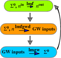
The flow chart in this QSGW tutorial was made with the script in the box below. The script is rather long but the parts that make the green, orange, and blue bubbles are all similar to one another. Cut and paste the content of the box below into file plot.qsgwcycle.
fplot
  -frme .0,.7,0,.7 -x -1,1 -y 0,1 -frmt th=2,3,3

# --- Green block ---
% var ys=1                 # position of block
% char filcol=.6,1,0       # color of bubble
  -lt 0,col=.5,.5,.5 -s square:fill=3:bold=103:col={filcol}:10.4,3.05 -tp 2~0,{ys}
  -lt 0,col=.5,.5,.5 -s circ:fill=3:bold=103:col={filcol}:3,90,270 -tp 2~-.50,{ys}
  -lt 0,col=.5,.5,.5 -s circ:fill=3:bold=103:col={filcol}:3,270,90 -tp 2~0.50,{ys}
  -lt 0,col=.5,.5,.5 -s square:fill=3:bold=-1:col={filcol}:10.8,2.8 -tp 2~0,{ys}
# ... text and arrow in green block
  -font b18
  -s arrow:fill=3:bold=3:col=.1,.1,1:-.07,0,.5,20,.4,.5 -tp 2~0+.04,{ys}-.01
  -lbl 0.03,{ys}:0 cc '~\{S}^\{0}, &\{n}^\{in}         &\{n}^\{out}'
  -font b16
  -lbl 0.04,{ys}+.03:0 cc 'lmf'
  -s arrow:fill=2:bold=4:col=.5,.5,.5:0,+.10,.5,30,.35,1 -tp 2~0+.04,{ys}-.09
  -s arrow:fill=2:bold=-1:col=.5,.5,.5:0,+.10,.5,30,.35,1 -tp 2~0+.04,{ys}-.09

# --- Orange block ---
% var ys=.7                # position of block
% char filcol=1,.6,0       # color of bubble
  -lt 0,col=.5,.5,.5 -s square:fill=3:bold=103:col={filcol}:12.47,3.05 -tp 2~0,{ys}
  -lt 0,col=.5,.5,.5 -s circ:fill=3:bold=103:col={filcol}:3,90,270 -tp 2~-.60,{ys}
  -lt 0,col=.5,.5,.5 -s circ:fill=3:bold=103:col={filcol}:3,270,90 -tp 2~0.60,{ys}
  -lt 0,col=.5,.5,.5 -s square:fill=3:bold=-1:col={filcol}:12.9,2.8 -tp 2~0,{ys}
# ... text and arrow in orange block
  -font b18
  -s arrow:fill=3:bold=3:col=.1,.1,1:-.12,0,.5,15,.4,.5 -tp 2~0-.12,{ys}-.02
  -lbl -.35,{ys}:0 lc '~\{S}^\{0}, &\{n}'
  -font b16
  -lbl 0.1,{ys}:0 rc 'GW inputs'
  -font b16
  -lbl -.15,{ys}+.03:0 cc 'lmfgwd'
  -s arrow:fill=2:bold=4:col=.5,.5,.5:0,+.10,.5,30,.35,1 -tp 2~0+.04,{ys}-.09
  -s arrow:fill=2:bold=-1:col=.5,.5,.5:0,+.10,.5,30,.35,1 -tp 2~0+.04,{ys}-.09

# --- Blue block ---
% var ys=.4                # position of block
% char filcol=0,.8,1       # color of bubble
  -lt 0,col=.5,.5,.5 -s square:fill=3:bold=103:col={filcol}:12.47,3.05 -tp 2~0,{ys}
  -lt 0,col=.5,.5,.5 -s circ:fill=3:bold=103:col={filcol}:3,90,270 -tp 2~-.60,{ys}
  -lt 0,col=.5,.5,.5 -s circ:fill=3:bold=103:col={filcol}:3,270,90 -tp 2~0.60,{ys}
  -lt 0,col=.5,.5,.5 -s square:fill=3:bold=-1:col={filcol}:12.9,2.8 -tp 2~0,{ys}
# ... text and arrow in blue block
  -font b16
  -s arrow:fill=3:bold=3:col=.1,.1,1:-.12,0,.5,15,.4,.5 -tp 2~0+.15,{ys}-.02
  -lbl -.70,{ys}:0 rc 'GW inputs'
  -font b18
  -lbl 0.4,{ys}:0 rc '~\{S}^\{0}'
  -font b16
  -lbl 0.15,{ys}+.03:0 cc 'lmgw'

# --- Arrow looping green to blue block : make stretched circle ---
  -ins 'gsave 1 4 scale .5 .5 .5 setrgbcolor'
#  no shift
#   -lt 0,col=0,0,0 -s circ:fill=0:bold=103:col=.5,1,0:3,290,90 -tp 2~.5+.2,.7-.99
#  -shftm=0,792-428
  -lt 0,col=0,0,0 -s circ:fill=0:bold=103:col=.5,1,0:3,290,90 -tp 2~.5+.2,.7-.99-1.083
  -ins 'grestore'
  -lt 0,bold=2 -s arrow:fill=3:col=0.5,0.5,0.5:.15/4,-.16/4,.99,25,.9 -tp 2~.68,1.01
$ fplot -shftm=0,792-428 -f plot.qsgwcycle
$ open fplot.ps
Note the use of -shftm to place the figure at the top of the page. This exercise explains how the shift was calculated.
Notes:
- Bubbles are assembled out of 4 parts: two half-circles, and two rectangles (the latter has no frame to blank out lines inside the bubble).
- Refer to the Symbols quick reference to see how the arrows are drawn and the Labels quick reference to see how the text is made.
- The long curved arrow was made with an arc (circle symbol), using
-lt 0,col=0,0,0 -s circ:fill=0:bold=103:col=.5,1,0:3,290,90 -tp 2~.5+.2,.7-.99-1.083
Explicit postscript was inserted (-ins ‘gsave 1 4 scale .5 .5 .5 setrgbcolor’) to stretch the arc.
Concept Index
Contour plots
| Instruction | Documentation | Example | |
|---|---|---|---|
| -con | DATA switches | Example 2.3 |
Data formats
| Documentation | Example | |
|---|---|---|
| default file structure | See notes on data format | Example 2.3 |
| instructions to specify file format | -r | |
| specify number of columns | -r:nc=n |
Error bars
| Instruction | Documentation/Example | Notes | ||
| -ey n | DATA switches, Error bar exercise | See also Symbols (-s) |
Fonts
| Instruction | Documentation | Example | Notes | |
|---|---|---|---|---|
| -font | LABELLING switches | |||
| roman | -font tn | Labels exercise | ||
| helvetica | -font hn | Labels exercise | ||
| italic | -font in | Labels exercise | ||
| bold | -font bn | Labels exercise | ||
| symbol | -font sn | |||
| size | -font tn | Labels exercise | ||
| change within a label | use {..} | Labelling and Numbering | Customize font in a portion of a label with curly brackets | |
| inside frames | -frme[:font=font] | Used only for frame numbering and labels. |
Frames
| Instruction | Documentation/Example | Notes | |
|---|---|---|---|
| -frme | FORMAT switches | ||
| size | -frme left,right,bottop,top | Frames Exercise | |
| font | -frme[:font=font] … | Frames Exercise | |
| fill color | -frme[:col=#,#,#] … | Frames Exercise | |
| suppress filling | -frme[:nofill] … | Frames Exercise | |
| nonorthogal axes | -frme[:theta=#] … | Frames Exercise | |
| log scale | -frme:lx|-frme:ly|-frme:lxy | Example 2.4 | See also Tic marks, log scale |
| graph paper | Frames Exercise | ||
| line type | -frmt | FORMAT switches | Frames Exercise |
| line thickness | -frmt th=# … | FORMAT switches | Frames Exercise |
| which axes | -frmt th=#,#,# … | Frames Exercise | |
| bounds | -x x1,x2 and -y y1,y2 | FORMAT switches | Example 2.4 |
| bounds, padding | -p# | FORMAT switches | Example 2.1, Example 2.4 |
Keys
| Instruction | Documentation/Example | ||
|---|---|---|---|
| -k | LABELLING switches | ||
| position | -k x,y … | Example 2.4 | |
| key line length | -k x,y:length | ||
| vertical spacing | -k x,y…,spacing … | Example 2.4 | |
| style | -k x,y…;style … | ||
| legend | -l strn … | DATA switches | Example 2.4 |
Labels
| Instruction | Documentation/Example | |
|---|---|---|
| -lbl | Labelling switches | |
| position | -lbl x,y … | Labels exercise |
| fill label box | -lbl x,y:0|:1 … | Labels exercise |
| justification | -lbl x,y cc … | Labels exercise |
| rotation | -lbl x,y cc,rot=# … | Labels exercise |
| group of labels | -lblx | -lbly | Labelling switches |
| abscissa | -xl string | Labelling switches, Labels exercise |
| ordinate | -yl string | Labelling switches, Labels exercise |
| title | -tl string | Labelling switches |
| labelling tic marks | See tic marks quick reference |
Line types
| Instruction | Documentation/Example | Notes | |
|---|---|---|---|
| solid, dashed, dotted lines_ | -lt n | DATA switches | |
| dash-dot lines | -lt 2~~#,#,#,# | Dot-dashed lines exercise | |
| color | -lt n~col=r,g,b | Example 2.4 | |
| thickness | -lt n~bold=# | Example 2.4 | |
| filling | -lt n~fill=# | ||
| clip outside frame | -lt n~clip | ||
| color weights | -lt n~colw=r,g,b | ||
| more color weights | -lt n~colwi=r,g,b | For color weights i=2|3|4, use ~colwi=ri,gi,bi | |
| split nonmonatomic data | -lt n~brk=1 |
Mapping and transformation of data
| Instruction | Documentation | Example | |
|---|---|---|---|
| columns for abscissa, ordinate | -col | DATA switches | |
| abscissa | -ab expr | DATA switches | |
| ordinate | -ord expr | DATA switches | Example 2.1 |
| multiple columns | -colsy | DATA switches | |
| rearrange or exclude data | -map | DATA switches | |
| interpolate | -itrp | DATA switches | Example 2.4 |
| sort abscissa | -sort | DATA switches |
Script files
| Instruction | Documentation | Example | |
|---|---|---|---|
| Read instructions from a file | -f file | INIT switches | Example 2.2 |
| Differences to command-line instructions | see Additional notes |
Symbols
| Instruction | Definition/Example | |
|---|---|---|
| -s type~options~shape-parameters | DATA switches | |
| types | -s +|x|circ|square|poly|wiggle|arrow|… | Symbols exercise |
| fill type | -s type~fill=# | Symbols exercise |
| fill color | -s type~col=r,g,b | Symbols exercise |
| line thickness | -s type~bold=b | Symbols exercise |
| clip | -s type~clip | |
| error bars | -ey n | DATA switches, Error bar exercise |
Tic marks
| Instruction | Definition/Example | Notes | |
|---|---|---|---|
| -tmx|-tmy spacing… | FORMAT switches | ||
| spacing | -tmx|-tmy spacing… | Frames Exercise | |
| No. tics /major tic | -tmx|-tmy spacing:mt | Frames Exercise | |
| placement | -tmx|-tmy spacing,pos | Frames Exercise | |
| major tic size | -tmx|-tmy spacing,rmt | Frames Exercise | |
| minor tic size | -tmx|-tmy spacing;rmnt | Frames Exercise | |
| for log scale | -tmx|-tmy spacing@2|@3|@4 | Example 2.4 | Use with -frme:lx|ly |
| user-specified | -tmx|-tmy spacing@5 | Example 2.4 | |
| numbering, suppress | -noxn|-noyn | LABELLING switches, Labels exercise | |
| numbering, format | -fmtnx|-fmtny | LABELLING switches, Labels exercise | |
| numbering, placement | -xn:t |-yn:r | LABELLING switches, Example 2.4 | |
| mapping | -abf expr | DATA switches |