The RPA and RPA+BSE Dielectric functions
This tutorial goes through how to add ladder diagrams to improve both the screened coulomb interaction , which improves the QSGW self-energy , and the macroscopic dielectric function . The random-phase approximation (RPA) to the macroscopic dielectric function can be also calculated very efficiently with the band code lmf; see this page for a detailed description. Whilst the dielectric function in the form produced by lmf is useful for detailed analysis, e.g. resolution of into individual k or band-pair contributions, there are two crucial effects missing. First, it neglects local fields; second there is no facility to go beyond the RPA and include electron-hole interaction effects. These effects can be included by adding ladder diagrams through the Bethe-Salpeter equation for the polarisation, as this tutorial demonstrates. See this page for a background to the theory.
This tutorial uses LiF as a simple test case. It is a highly polar system with a wide gap, which typically QS overestimates by 1 eV or so. This is largely because the electron-hole contributions that improve , also improve the screened coulomb interaction . As is well known, QS has a systematic tendency to overestimate bandgaps, the error increasing the gap. QS with ladder diagrams included in W largely ameliorates this error, and significantly improves the systematics of QS, as we show here for LiF. We will designate as W augmented with ladder diagrams.
In this tutorial, we will compare the QS and QS energy bands. Whether ladder diagrams are included or not, the QS procedure makes a quasiparticlized self-energy extracted from the fully dynamical , as explained in the introductory tutorial.
⟨ Create a fresh directory (mkdir lif && cd lif) and paste the structural information into init.lif ⟩
Make a self-consistent density within the LDA
blm init.lif --optics --brief --nk=4 --mix~nit=20 --gw~nvbse=4~ncbse=4 --ctrl=ctrl --autobas~ehmx=-.5 --rsham~el=-.5,-1.3~npr=50
echo --tbeh --v8 -vrsham=2 > switches-for-lm
lmfa lif `cat switches-for-lm`
lmf lif `cat switches-for-lm` > out.lmfsc
cp rst.lif rst-lda.lif
Make and plot the LDA energy bands
lmchk ctrl.lif  --syml~n=41~lblq:G=0,0,0,L=1/2,1/2,1/2,X=1,0,0,W=1,1/2,0,K=3/4,3/4,0~lbl=LGX
lmf ctrl.lif `cat switches-for-lm` --quit=rho
lmf ctrl.lif `cat switches-for-lm` --band~fn=syml
echo -5,20,5,10 | plbnds -fplot~scl=.5,.7 -ef=0 -scl=13.6 -lbl bnds.lif
cp bnds.lif bnds.blue
fplot -f plot.plbnds
Make a self-consistent QS self-energy
lmfgwd --job=-1 lif
touch bz.h5
rm -rf meta mixm.lif mixsigma *.h5
lmgw.sh ctrl.lif > lmgw.log
cp rst.lif rst-rpa.lif; cp sigm.lif sigm-rpa.lif
Make and plot the QS energy bands
lmf ctrl.lif `cat switches-for-lm` --quit=rho
lmf ctrl.lif `cat switches-for-lm` --band~fn=syml
echo -5,20,5,10 | plbnds -fplot~scl=.5,.7 -ef=0 -scl=13.6 -lbl bnds.lif
cp bnds.lif bnds.red
fplot -f plot.plbnds
Make a self-consistent QS self-energy
touch meta bz.h5; rm -r meta mixm.lif mixsigma
lmgw.sh --bsw ctrl.lif > bsw.log
cp rst.lif rst-bse.lif; cp sigm.lif sigm-bse.lif
Make and plot the QS energy bands
lmf ctrl.lif `cat switches-for-lm` --quit=rho
lmf ctrl.lif `cat switches-for-lm` --band~fn=syml
echo -5,20,5,10 | plbnds -fplot~scl=.5,.7 -ef=0 -scl=13.6 -lbl bnds.lif
cp bnds.lif bnds.green
fplot -f plot.plbnds
Make the RPA dielectric function
⟨ Edit the GWinput and ctrl files ⟩
lmfgwd --job=-1 lif
touch meta bz.h5
rm -r meta *.h5
cp rst-bse.lif rst.lif; cp sigm-bse.lif sigm.lif
echo --tbeh --v8 -vrsham=2 -vnkgw=8 > switches-for-lm
lmgw.sh -vnkgw=8 --epsq ctrl.lif > rpaoptics.log
mcx -r:h5~id=freq eps.h5 -s13.6 -r:h5~z~id=eps eps.h5 -real -r:h5~z~id=eps eps.h5 -s0,-1 -real -ccat -ccat > rpadat.8
fplot -frme 0,.7,0,.8 -x 0,22 -colsy 2 rpadat.8 -lt 2 -colsy 3 rpadat.8
Make the BSE dielectric function
⟨ Edit the GWinput and ctrl files ⟩
touch meta bz.h5
rm -r meta *.h5
echo --tbeh --v8 -vrsham=2 > switches-for-lm
lmgw.sh -veta1=.01 -vnkgw=8 --epsq --bse ctrl.lif > bseoptics.log
mcx -r:h5~id=freq epsbse.h5 -s13.6 -r:h5~z~id=eps epsbse.h5 -real -r:h5~z~id=eps epsbse.h5 -s0,-1 -real -ccat -ccat > bsedat.8
fplot -frme 0,1,0,1 -x 10,24 -colsy 3 bsedat.8  -lt 1,col=1,0,0 e2_experimental.dat
Preliminaries
Questaal executables such as blm, lmfa, lmf, lmfgwd, are all assumed to be in your path. The source code for all Questaal executables can be found here.
Tutorial
Start by making a fresh directory lif
mkdir lif && cd lif
Cut and paste the structural information in the box below into file init.lif.
HEADER Li F (Lithium fluoride)
LATTICE
# LiF lattice constant from https://link.springer.com/article/10.1007/BF01244483
# Cannot find T-dependence
% const a=4.0224
        SPCGRP=225 A={a}  UNITS=A
SPEC
   ATOM=F PZ=3.5 3.5
SITE
   ATOM=Li       X=     0.0000000    0.0000000    0.0000000
   ATOM=F        X=     0.5000000    0.5000000    0.5000000
Remark: Be sure that no spaces are interposed before the first column of init.lif, so that the categories like LATTICE and SITE begin in the leftmost column.
Note species declaration in init.lif. It tells the band code lmf to add high-lying local orbitals on the flourine s and p states. The input file maker (blm, below) will add them automatically anyway, but the is put there so you are aware of their importance. Leaving out the F 3s causes the LDA gap to be too large by 0.4 eV; including the F 3p state doesn’t affect the LDA that much but it changes the GW gap by a few tenths of an eV.
Now run blm to produce ctrl.lif.
blm init.lif --optics --brief --nk=4 --mix~nit=20 --gw~nvbse=4~ncbse=4 --ctrl=ctrl --autobas~ehmx=-.5 --rsham~el=-.5,-1.3~npr=50
Command-line switches are documented here. In particular:
--briefmakes an easy-to-read input file and sets up several parameters automatically--gwgenerates a category for QSGW calculations; and modifiers~nvbse=4~ncbse=4supply input to include 4 valence and 4 conduction states in the two-particle hamiltonian when calculating the BSE polarizability.--rsham~el=-.5,-1.3~npr=50prepares the ctrl file for a tight-binding form of the basis, a precursor to Jigsaw Puzzle Orbitals.--autobas~ehmx=-.5has no effect in this tutorial, but it is included in case you want to perform the calculation without a screened basis. (Materials with second-row elements need smooth hankel envelope functions somewhat deeper than usual to enable the QS self energy to interpolate smoothly between calculated k-points.)--opticsprepares the ctrl file to calculate the macroscopic dielectric function, .
One important thing to note are the parameters gcutb and gcutx. these are wave vector cut-offs used for the one-particle and two-particle sectors. The values blm chose are seen on this line
% const sig=12 gwemax=3.0 gcutb=3.6 gcutx=3.0 nvbse=4 ncbse=4 eta1=.02 eta2=eta1 # GW-specific
The values are reasonable, but they should be checked.
LDA calculation
With the ctrl, site, and basp files in hand (all autogenerated by blm), we can make a self-consistent LDA potential. Run lmfa first to generate the atomic densities (atm.lif), needed for a starting guess at the potential (Mattheis construction).
echo --tbeh --v8 -vrsham=2 > switches-for-lm
lmfa lif `cat switches-for-lm`
lmf lif `cat switches-for-lm` > out.lmfsc
cp rst.lif rst-lda.lif
The last line is not needed, but it preserves the LDA restart file for possible further exercises
Remarks: arguments --tbeh --v8 -vrsham=2 turn on the tight-binding form of the basis. The density should scarcely depend on whether or not they are used, but the tight-binding form makes the self-energy shorter ranged, which helps with interpolation. Packaging them in switches-for-lm seems a roundabout way to include these arguments on the command line, but the GW shell script used later on (lmgw.sh) knows about switches-for-lm, and will add them at appropriate places to various executables.
Turning to the output, observe that the LDA gap is about 8.9 eV (grep gap out.lmfsc), much smaller than the experimental gap (about 14.2-14.5 eV).
Now make and plot the energy bands (retain in file bnds.blue)
lmchk ctrl.lif  --syml~n=41~lblq:G=0,0,0,L=1/2,1/2,1/2,X=1,0,0,W=1,1/2,0,K=3/4,3/4,0~lbl=LGX
lmf ctrl.lif `cat switches-for-lm` --quit=rho
lmf ctrl.lif `cat switches-for-lm` --band~fn=syml
echo -5,20,5,10 | plbnds -fplot~scl=.5,.7 -ef=0 -scl=13.6 -lbl bnds.lif
cp bnds.lif bnds.blue
fplot -f plot.plbnds
View the postscript file with your favorite postscript reader, e.g. open fplot.ps on a Mac.
LDA energy bands for LiF. The experimental gap is about 14.2 eV.

Note the small dispersions in both valence and conduction bands. The heavy-hole p valence bandwidth is only 1 eV, compared to 3 eV in Si. These heavy masses, combined with the small dielectric constant, point to strong excitonic effects.
QSGW-RPA calculation
We now want to perform a QSGW calculation. To build the GWinput input file it requires, enter the following line:
lmfgwd --job=-1 lif
Warning: The GWinput file lmfgwd builds should be regarded only as a template — its parameters should always be checked — but it is sufficient in this case.
Make a self-consistent self-energy (QSGW level):
touch meta bz.h5; rm -rf meta mixm.lif mixsigma
lmgw.sh ctrl.lif > lmgw.log
cp rst.lif rst-rpa.lif; cp sigm.lif sigm-rpa.lif
(The first line is not needed for this step, but is put there to suggest safe practice; the last line is there to only retain information possibly used in later steps.)
lmgw.sh executes a sequence of steps through running a sequence of compiled executables; see the introductory tutorial.
Convergence should be reached after 6 iterations. grep more lmgw.log should produce something close to the following, which shows that the QSGW self-energy is well converged
lmgw: iter 1 of 99 completed in 24s, 25s from start. RMS change in sigma = 5.12e-2  Tol = 1e-5  more=T
lmgw: iter 2 of 99 completed in 25s, 50s from start. RMS change in sigma = 1.62e-2  Tol = 1e-5  more=T
lmgw: iter 3 of 99 completed in 24s, 74s from start. RMS change in sigma = 2.23e-3  Tol = 1e-5  more=T
lmgw: iter 4 of 99 completed in 22s, 96s from start. RMS change in sigma = 4.88e-4  Tol = 1e-5  more=T
lmgw: iter 5 of 99 completed in 22s, 118s from start. RMS change in sigma = 1.07e-4  Tol = 1e-5  more=T
lmgw: iter 6 of 99 completed in 21s, 139s from start. RMS change in sigma = 1.07e-5  Tol = 1e-5  more=T
lmgw: iter 7 of 99 completed in 21s, 160s from start. RMS change in sigma = 1.65e-6  Tol = 1e-5  more=F
Remarks:
The gap produced now should be about 15.9 eV (
grep gap llmf). This is significantly larger than the experimental gap (~14.2 eV), largely because of the missing ladder diagrams noted above, and it will reduce when ladders are added to the polarizability.QSGW widens the valence band slightly relative to LDA (bandwidth widens to 3.6 eV from 3.1 eV in the LDA case. It is notable that bandwidths widen relative to the LDA in wide-gap materials such as LiF and SrTiO3, while they narrow in correlated systems where the bandwidth is already small. In both cases QSGW significantly improves on the LDA.
There is a significant modification of the band gap owing to changes to the charge density. This is apparent in the output from lmf at the close of the starting iteration. Compare the gap in the first and last cycles of lmf as it iterates to charge self-consistency (
grep gap 1run/llmf; see discussion in the introductory tutorial). The widely used standard perturbative theory () misses this effect, which means if such a theory matches experiment well, the agreement is fortuitous. It is an important point, though rarely discussed. More detail can be found in this reference.
Make and plot the QSGW energy bands (retain in file bnds.red)
lmf ctrl.lif `cat switches-for-lm` --quit=rho
lmf ctrl.lif `cat switches-for-lm` --band~fn=syml
echo -5,20,5,10 | plbnds -fplot~scl=.5,.7 -ef=0 -scl=13.6 -lbl bnds.lif
cp bnds.lif bnds.red
fplot -f plot.plbnds
View the postscript file with your favorite postscript reader, e.g. open fplot.ps on a Mac.
QSGW energy bands of LiF. The experimental gap is about 14.2-14.5 eV.

QSGW-BSE self-energy
We can construct QS using QS as a starting point. (See Additional Exercise (1).) lmgw.sh is invoked in the same way to make QS as it is to make QS; only --bsw is added to the command line. (See this page for additional documentation on how to run lmgw.sh in BSE mode.)
touch meta bz.h5; rm -r meta mixm.lif mixsigma
lmgw.sh --bsw ctrl.lif > bsw.log
cp rst.lif rst-bse.lif; cp sigm.lif sigm-bse.lif
The first line removes memory of the original QS calculation. The last line is there to retain information for later steps. The second line clears out mixing files that keep prior iterations of the charge density (mixm.lif) and self-energy (mixsigma). (The BSE calculation generates a different so using prior iterations generated by the RPA calculation to accelerate convergence will only confuse the mixer.)
Note how lmgw.sh executes differently in the BSE case. In the RPA case
lmsig --tbeh --v8 -vrsham=2 ctrl.lif &> lsg ... 24s
instructions are replaced by the following
  lmsig --wrw-only   --tbeh --v8 -vrsham=2 ctrl.lif &> lx0  ... 9s
  bse  --tbeh --v8 -vrsham=2 ctrl.lif &> lbsw-b1  ... 133s
  lmsig --rdw    --tbeh --v8 -vrsham=2 ctrl.lif &> lsg  ... 14s
First it makes the RPA , which it needs to compute the BSE vertex. bse computes the two-particle hamiltonian and the BSE polarizability is calculated for every k point in the the Brillouin zone where it is needed to construct . bse overwrites the RPA with ; then lmsig can proceed in the usual manner, now with an improved . Note that bse is the rate-limiting step.
You might ask whether the vertex should be remade using a better () to construct it. This may be regarded as adding a specific set of higher order diagrams in many-body perturbation theory. Indeed lmgw.sh allows you to do this.
Compare how the RMS change in (actually ; see the introductory tutorial), converges to self-consistency (grep more bsw.log)
lmgw: iter 1 of 99 completed in 121s, 121s from start. RMS change in sigma = 1.35e-2  Tol = 1e-5  more=T
lmgw: iter 2 of 99 completed in 119s, 240s from start. RMS change in sigma = 3.96e-3  Tol = 1e-5  more=T
lmgw: iter 3 of 99 completed in 120s, 360s from start. RMS change in sigma = 1.1e-3  Tol = 1e-5  more=T
lmgw: iter 4 of 99 completed in 120s, 481s from start. RMS change in sigma = 2.42e-4  Tol = 1e-5  more=T
lmgw: iter 5 of 99 completed in 118s, 599s from start. RMS change in sigma = 9.01e-5  Tol = 1e-5  more=T
lmgw: iter 6 of 99 completed in 118s, 717s from start. RMS change in sigma = 1.47e-5  Tol = 1e-5  more=T
lmgw: iter 7 of 99 completed in 116s, 833s from start. RMS change in sigma = 1.17e-5  Tol = 1e-5  more=T
lmgw: iter 8 of 99 completed in 126s, 959s from start. RMS change in sigma = 7.7e-6  Tol = 1e-5  more=F
The initial RMS change in (1.35e-2) considerably smaller than we saw in 0th iteration starting from the LDA (5.12e-2). This implies that QS is a better description of the exchange-correlation potential than (assuming the QS potential is the most accurate). Nevertheless, convergence to self-consistency is slower. This is because the RPA has relatively unsophisticated short-range interactions (it does a rather poor job at short range), so adding ladder diagrams makes the structure of more complex. There is a greater disparity between the fast (high energy) and slow (low energy) degrees of freedom that put a larger burden on the mixer.
Inspect the QS bandgap (grep gap llmf). You should see that it comes out to about 14.8 eV. This is still larger than the experimental gap of 14.2 eV (Phys. Rev. B 13, 5530) to 14.5 eV (Solid State Commun. 17, 697). However, LiF has a large electron-phonon interaction; indeed a simple estimate of renormalization using a scheme based on Frolich’s original idea indicates that the electron-phonon interaction renormalizes the gap by about 0.5 eV, though it could be larger (see supplemental information to this paper). A better converged calculation gives a slightly smaller gap of 14.7 eV. With the various uncertainties it is not possible to precisely pin down how well the theory describes the gap, but agreement appears to be very good. LiF is typical: QS appears to describe one-particle properties very well in a wide range of insulators.
Also keep in mind that certain cutoff parameters may affect the result. For example, we used only 8 states for the BSE (nvbse=4 ncbse=4). Also there are the plane wave cutoffs (gcutb=3.6 gcutx=3.0). All of these need to be carefully checked.
Make and plot the QS energy bands (retain in file bnds.green)
lmf ctrl.lif `cat switches-for-lm` --quit=rho
lmf ctrl.lif `cat switches-for-lm` --band~fn=syml
echo -5,20,5,10 | plbnds -fplot~scl=.5,.7 -ef=0 -scl=13.6 -lbl bnds.lif
cp bnds.lif bnds.green
fplot -f plot.plbnds
QS energy bands of LiF. The experimental gap is about 14.2-14.5 eV.
If you have preserved the LDA, QS and QS energy bands in files bnds.blue, bnds.red, bnds.green respectively, you can combine the figures with the instructions shown below.
echo -5,20,5,10 | plbnds -fplot~scl=.5,.7 -ef=0 -dat=green -scl=13.6 -lbl green
echo -5,20,5,10 | plbnds -fplot~scl=.5,.7 -ef=0 -dat=red   -scl=13.6 -lbl red
echo -5,20,5,10 | plbnds -fplot~scl=.5,.7 -ef=0 -dat=blue  -scl=13.6 -lbl blue
mv plot.plbnds plot.plbnds~
echo "% char0 colg=1,bold=4,clip=1,col=.3,1,.2" >>plot.plbnds
echo "% char0 colr=3,bold=4,clip=1,col=1,.2,.3" >>plot.plbnds
echo "% char0 colb=2,bold=2,clip=1,col=.2,.3,1" >>plot.plbnds
awk '{if ($1 == "-colsy") {sub("-qr","-lt {colg} -qr");sub("blue","green");print;sub("green","red");sub("colg","colr");print;sub("red","blue");sub("colr","colb");print} else {print}}' plot.plbnds~ >> plot.plbnds
fplot -f plot.plbnds
Bands are colored according to the potential they are generated by. QS reduces the fundamental gap. This is a nearly universal feature of QS. Note the similarity in the QS and QS valence bands.

RPA macroscopic dielectric function
We can compute the macroscopic dielectric function in the RPA, following the steps of the introductory tutorial. We have a choice which hamiltonian to use to construct it. As is well known, peaks in are blue shifted, since the RPA omits electron-hole attraction (time dependent Hartree approximation). Diagrammatically, the bubbles should be augmented by attracting the electron and hole. That is how excitonic effects are expressed in diagrammatic language.
If we generate from a QS self-energy, the blue shift is compounded because the QS gap is overestimated. If we start instead from the LDA, the LDA gap underestimate redshifts and partially cancels the RPA error. Unfortunately, such a fortuitous cancellation merely obfuscates the various source of error. To disentangle the errors in the RPA from such effects, we start from the best self-energy available, the QS self-energy. Following the introductory tutorial reduce lcutmx in GWinput (not necessary, but the calculation runs more efficiently) Use your text editor or do sed -ibak s/'^ 4 *4/ 2 2/' GWinput to replace 4 with 2 in the second line shown :
lcutmx(atom) = l-cutoff for the product basis
 4 4
Remark: In 2022 and 2023 the algorithms and input for optics both changed considerably. For this section to work properly, you should compile from the repository a version dated Jan 2023 or newer. In particular the optics category should have the following tags
optics                               # Parameters for macroscopic dielectric function
      mode={loptic} npts=1001 window=0,1 mefac={mefac} ltet=1
      epsq=0,0,0.015  delre= 0.002 0.02
      bse[eta={eta1},{eta2} emesh=0,2,0.001]
To avoid the necessity of computing matrix elements of the position operator required for we pick a small q, slightly off zero. If q is chosen too small, there is a stability problem, and q=0.015 is a good compromise.\ Remark: There is also an option to compute for q=0, but as of this writing it relies on an approximate form of for the matrix elements of the position operator. See Exercise 4.
delre defines the energy mesh specifically for optics; it has the same meaning as delre in the GW category, the difference being the tag in OPTICS is used only for the optics branch. Typically you want a finer mesh for optics than what is needed to converge the self-energy, to resolve the peaks in . blm selected a default, which we will use here.
Compute for an 8×8×8 mesh
touch meta bz.h5
rm -r meta *.h5
cp rst-bse.lif rst.lif; cp sigm-bse.lif sigm.lif
lmgw.sh -vnkgw=8 --epsq ctrl.lif > rpaoptics.log
Extract in a standard Questaal format for 2D arrays.
mcx -r:h5~id=freq eps.h5 -s13.6 -r:h5~z~id=eps eps.h5 -real -r:h5~z~id=eps eps.h5 -s0,-1 -real -ccat -ccat > rpadat.8
Repeat for a 12×12×12 mesh:
rm -r meta *.h5
lmgw.sh -vnkgw=12 --epsq ctrl.lif > out.rpaeps
mcx -r:h5~id=freq eps.h5 -s13.6 -r:h5~z~id=eps eps.h5 -real -r:h5~z~id=eps eps.h5 -s0,-1 -real -ccat -ccat > rpadat.12
Compare the 8×8×8 and 12×12×12 meshes graphically:
fplot -frme 0,.7,0,.8 -xl E -yl eps -x 0,22 -y -1,5 -colsy 2 rpadat.8 -lt 2 -colsy 3 rpadat.8 -lt 1,col=1,0,0 -colsy 2 rpadat.12 -lt 2,col=1,0,0 -colsy 3 rpadat.12
View the postscript file with your favorite postscript reader, e.g. open fplot.ps on a Mac.
The two k meshes yield strikingly similar . This shows that is much less sensitive to the k mesh than Si is; in contrast to Si an 8×8×8 mesh is sufficient here.
RPA dielectric function generated from a QS self-energy, for an an 8×8×8 k mesh (black) and a 12×12×12 k mesh (red).

Note that is zero below the fundamental gap. Within the RPA (sometimes called — perhaps more appropriately — the time-dependent Hartree approximation) the bar polarizability is computed assuming particles are independent. Thus no excitonic effects are present and the optical gap and fundamental gap coincide at 15.2 eV.
Inspect from the first lines of rpadat.8 or rpadat.12. Both yield 1.70. (The precise number is hard to pin down because of difficulties in controlling cancelling divergences in the q→0 limit.) This is about 88% of the experimental value (~1.94), a bit larger than expected from the 80% rule. comes out a little smaller if we stick strictly to the RPA, that is, recover the QS self-energy (cp rst-rpa.lif rst.lif; cp sigm-rpa.lif sigm.lif) before running lmgw.sh. For the 8×8×8 mesh drops from 1.70 to 1.65. Also the shoulder for starts at a higher energy (15.9 eV instead of 14.8 eV). The reduction in and the blue shift in are related since the real and imaginary parts of are related via the Kramers Kronig relation (a condition for causality).
BSE macroscopic dielectric function
As in the RPA case, we have some choice which noninteracting hamiltonian to use when computing . The best choice is clearly QS; however, since QS is expensive to make, it is worthwhile to see how different is when generated from QS or from QS. See Additional Exercises (2). Here we consider only the QS case.
BSE optics uses the same two-particle basis as was used to make the self-energy, which is specifed in the GW category (gw_bse_nv and gw_bse_nc).
The raw BSE dielectric function consists of a set of discrete levels. To render a useful picture these must be broadened, as noted in the the introductory tutorial.
Broadening eta is specified in the OPTICS category of the ctrl file by tag
bse[eta={eta1},{eta2}]
Written in this form you specify bse_eta via the preprocessor variable eta1.
As shown above, there are two broadening parameters eta1 and eta2; however in this context only eta1 is active (the second one is used for q=0 optics). It turns out that, for LiF, choosing 0.01 Ry for eta1 yields a better resemblance to experimental data than the default value 0.02 Ry blm supplied (see Additional Exercises (3)).
Generate the BSE dielectric function for an 8×8×8 mesh and eta1=0.01 as follows:
touch meta bz.h5
rm -r meta *.h5
lmgw.sh -veta1=.01 -vnkgw=8 --epsq --bse ctrl.lif > bseoptics.log
is stored in epsbse.h5. Render in an ascii form with
mcx -r:h5~id=freq epsbse.h5 -s13.6 -r:h5~z~id=eps epsbse.h5 -real -r:h5~z~id=eps epsbse.h5 -s0,-1 -real -ccat -ccat > bsedat.8
We see that is 1.84, about 5% less than the experimental value. A calculation with better converged basis yields within 2% or so of experiment.
Compare to experimental data, digitized from D. M. Roessler and W. C. Walker, Optical constants of magnesium oxide and lithium fluoride in the far ultraviolet, J. Opt. Soc. Am. 57, 835 (1967). You can find the digitized experimental data in an ASCII file here.
fplot -frme 0,1,0,1 -x 10,24 -lt 1,col=1,0,0 e2_lif_experimental.dat -colsy 3 -lt 1,bold=4 bsedat.8
Imaginary part of the BSE dielectric function generated from a QS self-energy, for an an 8×8×8 k mesh (black) compared to experiment (red). For comparison, the light dashed lines show how the results change when a broadening eta1=0.02 is used (Exercise 3).

Agreement is strikingly good apart from apart from a uniform blue shift of 0.5 eV (see discussion on zero point motion, above), Peaks at 12.6, 14.5, 17.4, and 21.7 eV are well reproduced.
Before we run the bethesalpeter program we need to use lmf to produce the optical matrix elements, see this page for a description of how the optical matrix elements enter in to the expression for the macroscopic dielectric function. To do this we need to ensure the k-mesh used by bethesalpeter is consistent with that used by lmf. To do this run the following command
$ echo 6 | lmfgwd ctrl.lif
We then need to include information in ctrl.lif about which pairs of states etc to calculate the optical matrix elements for. We do this through the OPTICS category, see this page
OPTICS
  MODE=1
  LTET=0
  WINDOW=0.0 2.0
  NPTS=1001
  FILBND=1 4
  EMPBND=5 50
  MEFAC=0
MODE, LTET, WINDOW and NPTS do not affect the calculation of the matrix elements. FILBND and EMPBND include the upper and lower bounds on the valence and conduction bands for which we calculate the matrix elements and MEFAC determines how the contribution to these matrix elements from the non-local part of the potential is included. We do not include this correction here (it is handled in bethesalpeter, see below) hence MEFAC=0.
Next we run
$ lmf --opt:woptmc:permqp --revec:gw ctrl.lif --rs=1,0 -vnit=1
$ cp optdatac.lif optdatabse
where we copy the file produced to that read in by bethesalpeter. Before we perform the Bethe-Salpeter calculation we need to include some parameters in GWinput.
$ nano GWinput
The parameters for the calculation are
MaxOmega_BSE 2.0
MinOmega_BSE 0.0
numOmega_BSE 8000
NumValStates 4
NumCondStates 4
NLF_corr_BSE on
Qvec_bse 1 1 1  !q vector for BSE
ImagEner1 -0.083 !0.00160735
ImagEner2 0.107 !0.0138375
which are (in order of appearance): the maximum (in Rydberg) for which the dielectric function is calculated; the minimum ; the number of frequencies; the number of valence states to include in the Bethe-Salpeter equation; the number of conduction states included; LDA energies are used to construct the optical matrix elements accounting for a non-local potential; the direction of the perturbing field; Lorentzian broadening (Rydberg) at ; broadening at (broadening can increase linearly); do not read the kernel from a previous calculation; and do not read the diagonalized 2-particle Hamiltonian from a previous calculation. Note that NumValStates and/or NumCondStates can be less than the number of states included in FILBND and EMPBND in ctrl.lif. The valence and conduction states used in the Bethe-Salpeter equation are those closest to the Fermi level. The rest of the states are included in , but included at RPA level. The reason for doing this is the computational expense of solving the Bethe-Salpeter equation.
We are now ready to run a Bethe-Salpeter equation calculation to get the macroscopic dielectric function. To do this type
$ echo 0 | bethesalpeter > out.bse
$ cp eps_BSE.out eps_BSE.outBSE
eps_BSE.out contains parameters used, followed by three columns. The energy (for numOmegaBSE energies from MinOmega_BSE to MaxOmega_BSE) in eV are in column one followed by the real and imaginary parts of the macroscopic dielectric function. The imaginary part determines the absorption. We can vary the broadenings to match experiment. Ensure RestartwithKernel and RestartwithDiagonal are switched on to avoid having to calculate and diagonalize the matrix all over again.
Finally, the reason we copied the output file is so that we can compare this with an RPA . To do this type
$ echo -1 | bethesalpeter
The two outputs can be plotted in a plotting program such as gnuplot. The output from the two calculations above are shown below in the image, along with the experimental spectrum. 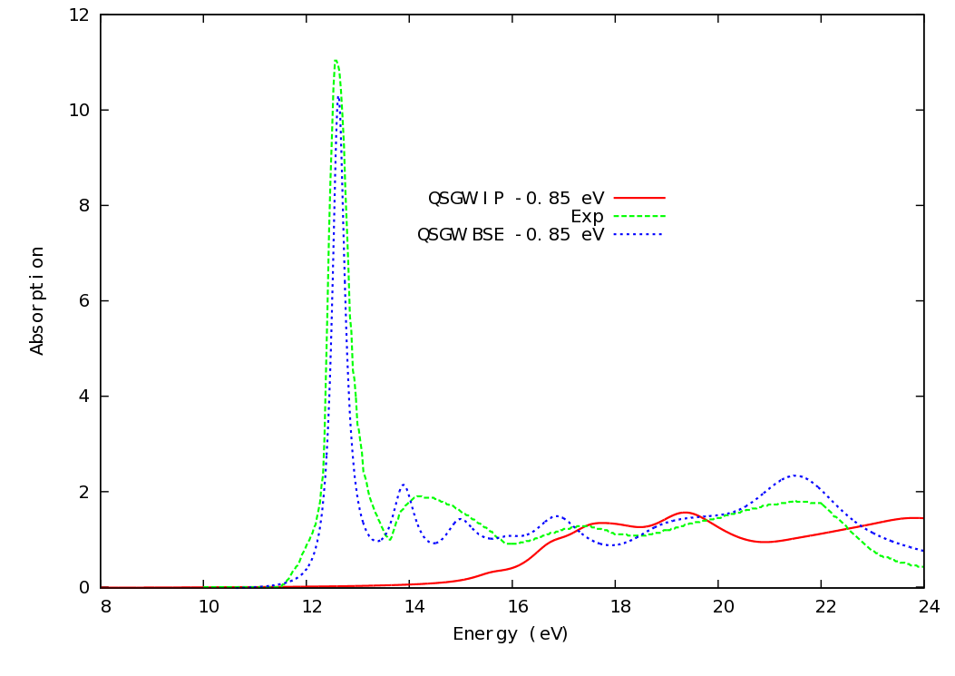
Adjust the broadenings to match experiment with RestartwithKernel and RestartwithDiagonal switched on.
Additional Exercises
1) Independence of starting point
At self-consistency QS (and also QS) are supposed to be independent of the starting potential. You can test whether it holds true here by generating the QS self-energy starting from QS or from the LDA.
2) Influence of input on
As noted in the RPA and BSE optics sections, there is some choice in which input to use in order to construct . Try making with taken from the LDA, taken from QS and from QS.
3) Role of broadening the BSE dielectric function
Comparing the BSE dielectric function to experiment in fine details can be deceiving, as the calculated result depends on how the function is smoothed. Try different smoothings and get a feel for what can be trusted and what is an artifact of the smoothing. In this instance, the calculation more closely resembles experimental data when a smoothing radius of 0.01 Ry is used. Try eta1=0.02 and see how the results change.
4) q=0 optics
Questaal has a branch that calculates optics in the q→0 limit. Since depends on the direction of approach to the origin, is not a scalar but a 3×3 tensor. As is customary, Questaal computes the diagonal (aka longitudinal) elements of the tensor, , and .
At present, Questaal can only calculate approximately. This is because it requires matrix elements of the position operator r. These matrix elements can be computed in terms of matrix elements of the (much simpler) momentum operator p only when the potential is local, as it is in density-functional theory. There is an approximation that becomes exact when the eigenfunctions of the nonlocal potential are the same as eigenfunctions of the local one. In that case the matrix elements of pnonloc can be computed by scaling ploc, and as of this writing questaal calculates in that approximation. To use this branch, invoke lmgw.sh as in the tutorial but without --epsq.
Note the following differences:
- The energy window and mesh spacing are defined by optics_bse_emesh (window between 0 and 2 Ry, with .001 Ry spacing in this case). optics_delre is not used.
- Both broadenings are active: broadening varies linearly in energy between the starting and final energies, starting with eta1 and ending with eta2 (both are are the same here unless you explicitly specify differently).
- is stored in an ascii file, eps-plot.txt. Both RPA and BSE response functions are written.
Compare the result to the small-q calculation. You should see that the two response functions are nearly the same up to about 16 eV; then the q=0 case peters out.
5) Running lmgw.sh in parallel
A scalar calculation will complete in a moderate time (10 minutes or less). You can do much better by using parallel constructs in lmgw.sh. This script runs heterogeneous parts, each of which can accept a unique set of parallel constructs. For that reason it has several switches to parallelize the several parts individually. (To see brief documentation of the switches lmgw.sh knows about, do lmgw.sh -h. See also the user guide.)
Here we will just select two switches: a generic one for scalar and another for parallel modes. Cores must be split between MPI and OMP/multithreading blocks. The switches below assume a single node with 16 cores, and it split the 16 cores into a 4×4 grid, for 4 MPI processes and 4 threads/process. The following variables also assume you have compiled the code with Intel’s MKL library.
Assuming you are running a bash shell, set shell variables
m1="env OMP_NUM_THREADS=16 MKL_NUM_THREADS=16 mpirun -n 1"
mn="env OMP_NUM_THREADS=4 MKL_NUM_THREADS=4 mpirun -n 4"
Repeat the calculation for the QSGW+BSE self-energy. You should get the same result, but with much faster execution, e.g. factor of 5 or so speedup. The lmgw.sh instruction would now read:
lmgw.sh --mpirun-1 "$m1" --mpirun-n "$mn" --bsw ctrl.lif > bsw.log
You can do still better by making pqmap files for both the RPA polarizability and the BSE polarizability. These files guide the GW code in its MPI parallelization over q-k combinations.
You can make the pqmap files by hand, but it is painful. It is easier to autogenerate them as follows.
lmfgwd lif `cat switches-for-lm` --lmqp~rdgwin --job=0 --batch~np=4~pqmap@plot
lmfgwd lif `cat switches-for-lm` --lmqp~rdgwin --job=0 --batch~np=4~pqmap@plot~bsw
The first command makes pqmap-4 a file for the RPA polarizability with 4 MPI processes, the second makes pqmap-bse-4 for the BSE polarizability. Repeat the BSE calculation as before.
Using maps will speed up lmgw.sh still more, but the the change is not dramatic because this system is too small to make much of an impact. On a standard X86 machine, You should see execution times of about 20 sec/iteration.
You can make a pqmap for the RPA part calculating the macroscopic dielectric function
lmfgwd lif -vnkgw=8 `cat switches-for-lm` --lmqp~rdgwin --job=0 --batch~np=4~pqmap@plot
You should remove pqmap-bse-4 since the BSE part is calculated for a particular q.