Introductory QSGW Tutorial

This tutorial provides a basic demonstration of a quasi-particle self-consistent GW (QSGW) calculation. Theory for GW and QSGW, and its implementation in the Questaal suite, can be found in references 1-5.

It begins with a calculation for Si in the local-density approximation (LDA). QSGW needs a starting point and usually relies on density-functional theory for it; but importantly, the final result should not depend on the starting point in QSGW,⁶ in contrast to standard (often referred to as 1-shot) GW calculations do. Self-consistency not only eliminates ambiguity in the starting point, it greatly improves the systematics and fidelity of GW. It also makes it possible to trace how diagrams missing from the theory systematically improve on the result. (The tradeoff is that QSGW is considerably more expensive than 1-shot GW.) An example of a 1-shot GW calculation is provided in a separate tutorial.

After a self-consistent self-energy is obtained, the energy bands are drawn, and the macroscopic dielectric function $\epsilon_M(\omega) = \left[\epsilon^{-1}_{G=0,G^\prime=0}(q{\rightarrow}0,\omega)\right]^{-1}$ is calculated in the random phase approximation (RPA). The calculated is repeated with the addition of ladder diagrams. Another tutorial explains how to calculate both the screened coulomb interaction $W$ and $\epsilon_M(\omega)$ with ladder diagrams.

nano init.si
blm init.si --optics --brief --nk=4 --mix~nit=20 --gw~nvbse=4~ncbse=4 --ctrl=ctrl --autobas~ehmx=-.5
lmfa si
lmf si > out.lmfsc

lmchk ctrl.si  --syml~n=41~lblq:G=0,0,0,L=1/2,1/2,1/2,X=1,0,0,W=1,1/2,0,K=3/4,3/4,0~lbl=LGXWGK
lmf ctrl.si --quit=rho
lmf ctrl.si --band~fn=syml
cp bnds.si bnds.blue

lmfgwd --job=-1 si
touch meta; rm -r meta
lmgwclear si
~/lmf/speedup/lmgw.mvs.sh --maxit=0 ctrl.si > lmgw.log

lmf ctrl.si --quit=rho
lmf ctrl.si --band~fn=syml
echo -13,10,5,10 | plbnds -fplot -ef=0 -scl=13.6 bnds.si
cp bnds.si bnds.red
fplot -f plot.plbnds
open fplot.ps

rm -f mixm.si
~/lmf/speedup/lmgw.mvs.sh  ctrl.si >> lmgw.log
lmf ctrl.si --band~fn=syml
cp bnds.si bnds.green

echo -13,10,5,10 | plbnds -fplot -ef=0 -scl=13.6 -dat=green -lbl green
echo -13,10,5,10 | plbnds -fplot -ef=0 -scl=13.6 -dat=red -lbl red
echo -13,10,5,10 | plbnds -fplot -ef=0 -scl=13.6 -dat=blue -lbl blue
mv plot.plbnds plot.plbnds~
echo "% char0 colg=1,bold=4,clip=1,col=.3,1,.2" >>plot.plbnds
echo "% char0 colr=3,bold=4,clip=1,col=1,.2,.3" >>plot.plbnds
echo "% char0 colb=2,bold=2,clip=1,col=.2,.3,1" >>plot.plbnds
awk '{if ($1 == "-colsy") {sub("-qr","-lt {colg} -qr");sub("blue","green");print;sub("green","red");sub("colg","colr");print;sub("red","blue");sub("colr","colb");print} else {print}}' plot.plbnds~ >> plot.plbnds
fplot -f plot.plbnds

rm -r meta
~/lmf/speedup/lmgw.mvs.sh -vnkgw=8  --epsq ctrl.si
mcx -r:h5~id=freq eps.h5 -s13.6 -r:h5~z~id=eps eps.h5 -real -r:h5~z~id=eps eps.h5 -s0,-1 -real -ccat -ccat > dat.8
fplot -frme 0,.7,0,.8 -x 1.5,6 -colsy 2 dat.8 -lt 2 -colsy 3 dat.8
open fplot.ps
rm -r meta
~/lmf/speedup/lmgw.mvs.sh -vnkgw=12 --epsq ctrl.si
mcx -r:h5~id=freq eps.h5 -s13.6 -r:h5~z~id=eps eps.h5 -real -r:h5~z~id=eps eps.h5 -s0,-1 -real -ccat -ccat > dat.12
rm -r meta
~/lmf/speedup/lmgw.mvs.sh -vnkgw=16 --epsq ctrl.si
mcx -r:h5~id=freq eps.h5 -s13.6 -r:h5~z~id=eps eps.h5 -real -r:h5~z~id=eps eps.h5 -s0,-1 -real -ccat -ccat > dat.16
fplot -frme 0,.7,0,.8 -x 1.5,6 -colsy 2 dat.8 -lt 2 -colsy 3 dat.8 -lt 1,col=1,0,0 -colsy 2 dat.12 -lt 2,col=1,0,0 -colsy 3 dat.12 -lt 1,col=0,1,0 -colsy 2 dat.16 -lt 2,col=0,1,0 -colsy 3 dat.16

rm -r meta
~/lmf/speedup/lmgw.sh -vnkgw=8 --epsq --bse ctrl.si > bse.log
mcx -r:h5~id=freq epsbse.h5 -s13.6 -r:h5~z~id=eps epsbse.h5 -real -r:h5~z~id=eps epsbse.h5 -s0,-1 -real -ccat -ccat > bsedat.8
fplot -frme 0,.7,0,.8 -x 1.5,6 -colsy 2 bsedat.8 -lt 2 -colsy 3 bsedat.8

rm -r meta
mn="env OMP_NUM_THREADS=4 MKL_NUM_THREADS=4 mpirun -n 4"
~/lmf/speedup/lmgw.sh -vnkgw=12 --mpirun-n "$mn" --epsq --bse ctrl.si > bse.log

Introduction

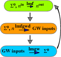
Each iteration of a QSGW calculation has two main parts: a section that uses effective one-body hamiltonians to make the density n (as in DFT; only now the generating potential does not depend on n alone), and the GW code that makes the self-energy $\Sigma(\omega)$ of an interacting hamiltonian. For quasiparticle self-consistency, the GW code makes a “quasiparticlized” self-energy $\Sigma^0$, which is used to construct the effective one-body hamiltonian for the next cycle. The process is iterated until the change in $\Sigma^0$ becomes small. Usually the interacting $\Sigma(\omega)$ isn’t made explicitly, but you can do so, as explained in this tutorial. See References 1-5 for a discussion of QSGW and Questaal’s implementation of it.

In Questaal the one-body executable is lmf. The script lmfgwd is similar to lmf, but it is a driver whose purpose is to set up inputs for the GW code. $\Sigma^0$ is made by a shell script lmgw.sh, which runs the cycle shown in the figure above. It also does some bookkeeping, such as monitoring convergence to self-consistency. (In the classic code, lmgwsc plays the role of lmgw.sh, which is a wrapper for script lmgw that calls the relevant compiled codes.)

This tutorial also uses some auxiliary utilities, e.g. plbnds and fplot. Postscript files can be rendered by your favorite postscript viewer, here assumed for purposes of demonstration the Apple open utility.

Before any self-energy $\Sigma^0$ exists, it is assumed to be zero. Thus the one-body hamiltonian is usually the LDA, though it can be something else, e.g. LDA+U⁷. We call the cycle before $\Sigma^0$ exists the “zero^th iteration.”

At any step in the cycle there are two self-energies and two corresponding Green’s functions: the interacting $G[\Sigma(\omega)]$ and non-interacting $G^0[\Sigma^0]$. At self-consistency the poles of $G$ and $G^0$ coincide: this is a unique and very advantageous feature of QSGW. It means that there is no “mass renormalization” of the bandwidth — at least at the GW level. Indeed the QSGW energy bands can be wider than bands given by density-functional theory, as in Ref 8. In correlated materials, they are typically narrower; see for example Ref 9.

In short, a QSGW calculation consists of the following steps. The starting point is a self-consistent DFT calculation (usually LDA). The DFT eigenfunctions and eigenvalues are used by the GW code to construct a self-energy $\Sigma^0$. This is called the “0^th iteration.” If only the diagonal parts of $\Sigma^0$ are kept, the “0^th” iteration corresponds to what is sometimes called 1-shot GW, or as G^LDAW^LDA.

In the next iteration, $\Sigma^0-V_{xc}^\text{LDA}$ is added to the LDA hamiltonian. The density is made self-consistent, and control is handed over to the GW part. (Note that for a fixed density $V_{xc}^\text{LDA}$ cancels the exchange-correlation potential from the LDA hamiltonian.) This process is repeated until the RMS change in $\Sigma^0$ falls below a certain tolerance value. The final self-energy (QSGW potential) can be thought of as an effective exchange-correlation functional that is tailored to the system. This is very convenient as it can now be used in an analogous way to standard DFT to calculate properties such as the band structure.

Note: The main GW algorithm has been completely redesigned by D. Pashov. It is much more efficient and makes extensive use of MPI, OPENMP, and multithreading. It has also been adapted to run efficiently on NVidia A100 and V100 GPU’s. In this tutorial we will use the current code, but also present instructions for the classic implementation.

Preliminaries

This tutorial assumes you have downloaded the repository (see this page for instructions on getting access to and downloading the Questaal package), that you have built (compiled) the executable codes and installed them in a some directory in your path, e.g. ~/bin.

The source code for all Questaal executables can be found here.

LDA calculation

The starting point is a self-consistent LDA density, and proceeds in almost the same way as the introductory DFT tutorial for silicon. The starting input is the same. Copy the following lines to file init.si):

LATTICE
# ALAT is a length scale, in atomic units
        ALAT=10.26
# PLAT refers to primitive lattice vectors, in units of alat
        PLAT=    0.00    0.50    0.50
                 0.50    0.00    0.50
                 0.50    0.50    0.00
# POS refers to cartesian coordinates, in units of alat
SITE
     ATOM=Si   POS=    0.00    0.00    0.00
     ATOM=Si   POS=    0.25    0.25    0.25

Run the following commands to obtain a self-consistent density:

blm init.si --optics --brief --nk=4 --mix~nit=20 --gw,nk=3 --ctrl=ctrl
lmfa si
lmf si > out.lmfsc

In contrast to the basic tutorial, blm includes an extra --gw switch, which tailors the ctrl file for a GW calculation. To see how it affects the ctrl file, try running blm without --gw. The switch modifies the basis set section (see the AUTOBAS line) to increase the size of the basis, which is necessary for GW calculations.

Two new blocks of text, the HAM and GW categories, are also added towards the end of the ctrl file. The extra parameters in the HAM category handle the inclusion of a quasiparticlized GW self-energy $\Sigma^0$. The GW category provides some default values for parameters that are required in the GW calculation. The GW code has its own input file and the DFT ctrl file influences what defaults are set in it, we will come back to this later.

Note: In practice the usual LDA hamiltonian is made with a local exchange correlation potential $V_{xc}^\text{LDA}$, and $\Sigma^0-V_{xc}^\text{LDA}$ is added to it. This useful because as the density changes, the change in the LDA potential ${\delta}V_{xc}^\text{LDA}$, is a reasonable proxy for the change $\delta\Sigma^0$ in $\Sigma^0$; thus $\delta\Sigma^0-{\delta}V_{xc}^\text{LDA}$ should be smaller than $\delta\Sigma^0$.

Now check the output file out.lmfsc. It should converge in 10 iterations as can be seen from grep DQ out.lmfsc. Note that ehf and ehk should be essentially the same (-1156.140505 Ry); see the end of out.lmfsc or inspect save.si.

Look for the bandgap (grep gap out.lmfsc). It should be around 0.58 eV. Note that, because we used a coarse mesh of 4×4×4 k points, the closest conduction band minimum to the actual minimum on this mesh is at X. Thus what is printed is the gap between Γ and X, not the true minimum gap, which occurs on the Γ-X line (see this tutorial and is slightly smaller. In any case it is well below the the experimental gap (1.2 eV).

Now that we have the input eigenfunctions and eigenvalues, the next step is to carry out a GW calculation. Before moving on to the GW calculation, let’s make the LDA energy bands. lmf requires a symmetry lines file. We’ll chose the popular sequence L,Γ,X,W,ΓK (we are just tracing the same steps in the LDA tutorial). Make the symmetry-lines file this way (syml.si)

lmchk ctrl.si  --syml~n=41~lblq:G=0,0,0,L=1/2,1/2,1/2,X=1,0,0,W=1,1/2,0,K=3/4,3/4,0~lbl=LGXWGK

Aside: If you need to see or remember what a particular command-line switch does, you can either run the executable with --h, which supplies minimal information, or see the command-line arguments web page For the --syml switch this documentation just points to another page where it is explained in more detail.

Make the bands as follows:

lmf ctrl.si --quit=rho                        ← makes a pass without changing the density: sets the Fermi level
lmf ctrl.si --band~fn=syml
cp bnds.si bnds.blue                          ← save it so we can compare to GW

To view the LDA bands, see this tutorial. For now we’ll defer drawing figures until we have GW results to compare with.

How lmf incorporates GW self-energies

lmf is code that implements density functional theory. But it also can read a (quasiparticlized) self-energy $\Sigma^0$ (more accurately, $\Sigma^0{-}V_{xc}^\text{LDA}$), which it adds to the $V_{xc}^\text{LDA}$. With this addition most of the functions performed at the LDA level can also be performed at the QSGW level.

The GW scheme computes $\Sigma^0$ in the band representation, i.e. as $\Sigma^0_{n,n'}(\mathbf{k})$. $\Sigma^0$ can also be rotated to the orbital basis, $\Sigma^0_{\mathbf{R}i,\mathbf{R'}i'}(\mathbf{k})$. In Questaal’s basis set, basis functions are centered at some site $\mathbf{R}$ in the unit cell, and each site has multiple orbitals, labelled $i$. $\Sigma^0$ is stored on disk in this representation (file sigm.ext).

The GW code must calculate $\Sigma^0(\mathbf{k})$ at specific k points; however, lmf has a very handy scheme to interpolate $\Sigma^0(\mathbf{k})$ to any k. Roughly speaking, $\Sigma^0_{\mathbf{R}i,\mathbf{R'}i'}(\mathbf{k})$ is inverse Bloch transformed to a real-space form, $\Sigma^0_{\mathbf{(R+T)}i,\mathbf{R'}i'}$. $\Sigma^0_{\mathbf{R}i,\mathbf{R'}i'}(\mathbf{k})$ can be evaluated for any k by a forward Bloch transform of $\Sigma^0_{\mathbf{(R+T)}i,\mathbf{R'}i'}$ at the desired k. The real algorithm is somewhat more complicated, but this is the main idea. This facility is extremely useful: it is possible to put the QSGW potential on the same footing as a density-functional potential — able to generate energy bands or other properties on an arbitrary mesh.

Note: the k-mesh for $\Sigma^0(\mathbf{k})$ (read from GW_NKABC) is distinct from the k mesh lmf uses for Brillouin zone integrations (read from BZ_NKABC). This is possible to do because of the interpolation scheme just noted. Typically a coarser mesh can often be used for $\Sigma^0(\mathbf{k})$ because it varies more smoothly than the rest of the hamiltonian (kinetic energy especially). For that reason it is not necessary to evaluate $\Sigma^0(\mathbf{k})$ on as fine a k mesh as lmf requires, e.g. to make Brillouin zone integrations for the density-of-states or the charge density. This is fortunate because the work needed to generate $\Sigma^0(\mathbf{k})$ is much greater than the work lmf needs to generate the rest of the hamiltonian. (In the existing implementation the computation time to make $\Sigma^0(\mathbf{k})$ scales as (number-of-k-points)²). Through the relation between real- and reciprocal- space representations of $\Sigma^0$, it is apparent that the number of k points needed for $\Sigma^0$ in k space is related to the range of $\Sigma^0$ in real space.

This tutorial selected a k mesh of 3×3×3 divisions on which make $W$ and the self-energy, $iGW$. This mesh is a bit rough, but it makes the calculation fast and for Si the results are reasonable. In this tutorial we will stick with 3 k divisions, but you need to monitor the k convergence. This can be time consuming and unfortunately there are no shortcuts.

GW_GCUTX controls the plane wave cutoff of the two-particle basis. The computational cost is sensitive to this value, so you want to make it as low as possible without messing up the results. It is a good idea to try a couple of values to satisfy yourself that you have made a sensible choice: make it as small as you can while keeping the QP levels reasonable well converged.

In correlated cases the mixing parameter beta for the self-energy, analogous to the mixing parameter beta for the charge density, that controls how much of the current iteration is to be admixed with prior ones, need to be reduced. It is controlled by GW_MIXBETA.

Other convergence parameters to particularly watch out for are the product basis tolerance, the augmentation lcutmx, and whether product basis functions are included for shallow core states. The GWinput file is documented on this page.

Running QSGW

We are now ready for a QSGW calculation, which you do with the shell script lmgw.sh: further documentation for lmgw.sh can be found on this page.

lmgwclear si
lmgw.sh --maxit 2  ctrl.si

lmgwsc --wt --insul=4 --tol=2e-5 --maxit=0 si        &larrr; zeroth iteration of QSGW calculation

lmgw 14:14:45 : invoking mpirun -n 1 lmf --no-iactive  si >llmf

    lmgw 14:15:37 : invoking mpirun -n 1 rdata4gw_v2 --job=0 --legacy=0  >lrdata4gw
    lmgw 14:15:37 : invoking mpirun -n 1 heftet --job=1 >leftet
    lmgw 14:15:37 : invoking mpirun -n 1 hchknw --job=1 >lchknw
    lmgw 14:15:38 : invoking mpirun -n 1 hbasfp0 --job=3 >lbasC
    lmgw 14:15:38 : invoking mpirun -n 1 hvccfp0 --job=0 >lvccC ... 0.0m (0.0h)
    lmgw 14:15:40 : invoking mpirun -n 1 hsfp0_sc --legacy=0 --job=3 >lsxC ... 0.0m (0.0h)
    lmgw 14:15:40 : invoking mpirun -n 1 hbasfp0 --job=0  >lbas
    lmgw 14:15:41 : invoking mpirun -n 1 hvccfp0 --job=0 >lvcc ... 0.0m (0.0h)
    lmgw 14:15:43 : invoking mpirun -n 1 hsfp0_sc --legacy=0 --job=1 >lsx ... 0.0m (0.0h)
    lmgw 14:15:43 : invoking mpirun -n 1 hx0fp0_sc  --job=11 >lx0 ... 0.1m (0.0h)
    lmgw 14:15:47 : invoking mpirun -n 1 hsfp0_sc --legacy=0 --job=2  >lsc ... 0.1m (0.0h)
    lmgw 14:15:53 : invoking mpirun -n 1 hqpe_sc --legacy=0 4 >lqpe ... 0.0m (0.0h)

The self-energy produced so far is essentially the same as G^LDAW^LDA generated in the one-shot tutorial, only now there is no Z factor and the full $\Sigma^{nn^\prime}$ is generated. This is distinct from computing the level shift in first=order perturbation theory as lmgw1-shot did (and most GW codes do). This requires only the diagonal $\Sigma^{nn}$, which is faster and easier to make (and is why QSGW is more expensive to do).

Even though it is standard practice to use a Z factor in 1-shot GW, in the Appendix of reference 1 we explain why it is better to use Z=1 even in the 1-shot case. (It is a poor man’s version of self-consistency.) Finally, in the self-consistent case the Z factor makes no sense because the input and output quasiparticle levels are the same.

Inspect the output of lmgw.sh

recording execution environment to file env
  16:57:57 env > env
    starting iteration 1 of 2
  16:57:57 lmfgwd --job=0 --lmqp~rdgwin --gwcode=2 --no-iactive ctrl.si &> llmfgw00			← Makes some setup files, e.g. the list of k points
  16:57:57 lmfgwd --job=1 --gwcode=2 --no-iactive ctrl.si &> llmfgw01  ... 1s				← Makes eigenfunctions and some matrix elements for GW
  16:57:58 rdata4gw_v2 --job=0 --efmode=1 --chknwmode=1 ctrl.si &> lrdata4gw				← Translates some files into formats the GW recognizes
  16:57:58 hbasfp0 --job=3 --ppbfl=ppbrdc.h5 ctrl.si &> lbasC						← Makes the product basis for the core partial waves
  16:57:58 hbasfp0 --job=0 ctrl.si &> lbas  ... 1s							← Makes the product basis for the valence partial waves
  16:57:59 hvccfp0 --ppbfl=ppbrdc.h5 --vcfl=vcc.h5 ctrl.si &> lvccC  ... 1s				← Makes the Hartree potential for the core
  16:58:00 hvccfp0 ctrl.si &> lvcc  ... 1s								← Makes matrix elements of the Hartree potential
  16:58:01 hsfp0_sc ctrl.si &> lsxC									← Makes the Hartree-Fock exchange potential for the core
  16:58:01 lmsig ctrl.si &> lsg  ... 6s									← Makes the self-energy and writes Sigma0
... rms change in sigma: 1.11e-3, tol: 1e-5.								← Prints the RMS change in Sigma0 from prior iteration
  16:58:07 rm -f mixm.si
  16:58:07 lmf ctrl.si &> llmf  ... 1s									← Makes the density self-consistent for an updated Sigma0
  16:58:08 save_iter "1run" "llmf llmfgw_0 llmfgw00 llmfgw01 llmfgw02 llmf02 lrdata4gw lbasC lvccC lsxC lbas lvcc lx0 lw0 lbsw-b* lbse lsg lqpe sig.h5 sigm sigm.si beff.si bnds.si save.si rst.si ctrl.si site.si basp.si atm.si GWinput switches-for-lm bse-flags lmsig-flags tol c4tol c4maxit maxit"
lmgw: iter 1 of 1 completed in 11s, 11s from start. RMS change in sigma = 1.11e-3  Tol = 1e-5  more=F

Note the last step: lmf was invoked to make a new charge density in the presence of a fixed $\Sigma^0{-}V_{xc}^\text{LDA}$. In the absence of self-consistency, there is an ambiguity as to whether the original density or the updated one should be used to interpret results. (If only the diagonal part of $\Sigma^0$ is retained, as is usual in 1-shot calculations, the addition of $\Sigma^0$ doesn’t change the density: only the QP levels change).

RDSIGM: read file sigm and create COMPLEX sigma(R) by FT ...

 mixrho:  sought 2 iter, 3182 elts from file mixm; read 0.  RMS DQ=6.65e-4

 VBmax = 0.160399  CBmin = 0.252678  gap = 0.092278 Ry = 1.25499 eV
...
 VBmax = 0.159132  CBmin = 0.253739  gap = 0.094607 Ry = 1.28665 eV

Before continuing, let’s make and preserve the energy bands from the 0^th iteration.

lmf ctrl.si --quit=rho                       # makes a pass without changing the density: sets Ef in moms.si
lmf ctrl.si --band~fn=syml
cp bnds.si bnds.red                          # save it so we can compare to other bands

Iterating QSGW to self-consistency, preliminary considerations

Remarks regarding iterations to self-consistency:

You can skip this section you just want to get on with the tutorial. However, the points below are important things to keep in mind if you want to make the best use of lmgw.sh.

1. As it executes, lmgw.sh records the iteration it is in and whatever instruction it executes wthin that iteration. Thus, if a calculation is aborted it can restart where the last calculation left off. This information is in directory meta. Inspect the directory (ls meta/) and you will find only one file, meta/iter. Once all the intermediate steps of an iteration are completed, meta is cleared except for the iterations counter (the contents of meta/iter should be 1 for now). If you don’t want lmgw.sh to remember its history, simply remove this directory.

2. Two self-energy files are present, sigm.si and sig.h5. Eventually these will be merged into one file, but for now, note that sig.h5 is used by lmgw.sh and sigm.si is written only at the end of the cycle, to maintain compatibility with lmf. The two files are now in sync, so it doesn’t matter in the present case; however if you start from a directory containing only the sigm file, you should make a corresponding sig.h5. Do this with: ln -s sigm.si sigm; s2s5; rm sigm. (Having sig.h5 is only important at the end of the cycle, when self-energies are mixed).

3. If you did not start the calculation from a fresh directory, you should remove all files *.h5 except retain or remake sig.h5.

4. This tutorial runs quickly, so parallelization is not needed. But lmgw.sh enables a high degree of parallelization, and you will need to make use of it when running larger calculations.

Iterating QSGW to self-consistency

Rerun lmgw.sh, this time not restricting the number of iterations

rm -f mixm.si

m1="env OMP_NUM_THREADS=16 MKL_NUM_THREADS=16 mpirun -n 1"
mn="env OMP_NUM_THREADS=4  MKL_NUM_THREADS=4  mpirun -n 4" 

lmgw.sh --incount --mpirun-1 "$m1" --mpirun-n "$mn" --tol=2e-5 ctrl.si &> lmgw.log &

Inspect lmgw.log (grep RMS lmgw.log) to monitor convergence to self-consistency

lmgw: iter 2 of 100 completed in 7s, 7s from start. RMS change in sigma = 1.98e-4  Tol = 2e-5  more=T
lmgw: iter 3 of 100 completed in 6s, 13s from start. RMS change in sigma = 3.58e-5  Tol = 2e-5  more=T
lmgw: iter 4 of 100 completed in 7s, 20s from start. RMS change in sigma = 6.37e-6  Tol = 2e-5  more=F

The RMS change in $\Sigma^0$ rapidly dropped to a small number. We have reached self-consistency in $\Sigma^0$. Look also at the RMS change in the density at the last iteration. You should see that the $n[\Sigma^0]$ is essentially identical to $n[\Sigma^0]$ from the prior iteration (grep RMS ./?run/llmf)

./0run/llmf: mixrho:  sought 2 iter, 4070 elts from file mixm; read 0.  RMS DQ=2.96e-6
./0run/llmf: mixrho:  sought 2 iter, 4070 elts from file mixm; read 1.  RMS DQ=2.23e-6  last it=2.96e-6
./1run/llmf: mixrho:  sought 2 iter, 4070 elts from file mixm; read 0.  RMS DQ=7.60e-4
./1run/llmf: mixrho:  sought 2 iter, 4070 elts from file mixm; read 1.  RMS DQ=5.16e-4  last it=7.60e-4
./1run/llmf: mixrho:  sought 2 iter, 4070 elts from file mixm; read 2.  RMS DQ=2.59e-5  last it=5.16e-4
./1run/llmf: mixrho:  sought 2 iter, 4070 elts from file mixm; read 3.  RMS DQ=1.92e-5  last it=2.59e-5
./2run/llmf: mixrho:  sought 2 iter, 4070 elts from file mixm; read 0.  RMS DQ=5.33e-5
./2run/llmf: mixrho:  sought 2 iter, 4070 elts from file mixm; read 1.  RMS DQ=2.93e-5  last it=5.33e-5
./3run/llmf: mixrho:  sought 2 iter, 4070 elts from file mixm; read 0.  RMS DQ=1.53e-5
./3run/llmf: mixrho:  sought 2 iter, 4070 elts from file mixm; read 1.  RMS DQ=9.97e-6  last it=1.53e-5
./4run/llmf: mixrho:  sought 2 iter, 4070 elts from file mixm; read 0.  RMS DQ=1.15e-6
./4run/llmf: mixrho:  sought 2 iter, 4070 elts from file mixm; read 1.  RMS DQ=8.01e-7  last it=1.15e-6

Thus at self-consistency, both $\Sigma^0$ and the density stop changing, ameliorating ambiguity in, e.g. the Fermi level. QSGW is not a conserving approximation as fully self-consistent GW is, but it is fairly close to a conserving one, and indeed it vastly better than one-shot GW. Morever, QSGW can provide very useful ground state properties, e.g. the charge density. Charges and magnetic moments are generally not accessible in standard G^LDAW^LDA.

Check the band gap evolution during the different iterations (grep gap ./?run/llmf)

./0run/llmf: VBmax = 0.162578  CBmin = 0.205082  gap = 0.042504 Ry = 0.57830 eV
./1run/llmf: VBmax = 0.160540  CBmin = 0.252664  gap = 0.092125 Ry = 1.25342 eV
./1run/llmf: VBmax = 0.160540  CBmin = 0.252664  gap = 0.092125 Ry = 1.25342 eV
./1run/llmf: VBmax = 0.160267  CBmin = 0.252883  gap = 0.092615 Ry = 1.26009 eV
./1run/llmf: VBmax = 0.160267  CBmin = 0.252883  gap = 0.092615 Ry = 1.26009 eV
./1run/llmf: VBmax = 0.159670  CBmin = 0.253378  gap = 0.093709 Ry = 1.27497 eV
./1run/llmf: VBmax = 0.159670  CBmin = 0.253378  gap = 0.093709 Ry = 1.27497 eV
./1run/llmf: VBmax = 0.159650  CBmin = 0.253433  gap = 0.093784 Ry = 1.27599 eV
./1run/llmf: VBmax = 0.159650  CBmin = 0.253433  gap = 0.093784 Ry = 1.27599 eV
./2run/llmf: VBmax = 0.159700  CBmin = 0.257482  gap = 0.097782 Ry = 1.33040 eV
./2run/llmf: VBmax = 0.159700  CBmin = 0.257482  gap = 0.097782 Ry = 1.33040 eV
./2run/llmf: VBmax = 0.159669  CBmin = 0.257512  gap = 0.097843 Ry = 1.33122 eV
./2run/llmf: VBmax = 0.159669  CBmin = 0.257512  gap = 0.097843 Ry = 1.33122 eV
./3run/llmf: VBmax = 0.158704  CBmin = 0.258781  gap = 0.100077 Ry = 1.36162 eV
./3run/llmf: VBmax = 0.158704  CBmin = 0.258781  gap = 0.100077 Ry = 1.36162 eV
./3run/llmf: VBmax = 0.158708  CBmin = 0.258753  gap = 0.100045 Ry = 1.36118 eV
./3run/llmf: VBmax = 0.158708  CBmin = 0.258753  gap = 0.100045 Ry = 1.36118 eV
./4run/llmf: VBmax = 0.158589  CBmin = 0.258881  gap = 0.100292 Ry = 1.36454 eV
./4run/llmf: VBmax = 0.158589  CBmin = 0.258881  gap = 0.100292 Ry = 1.36454 eV
./4run/llmf: VBmax = 0.158589  CBmin = 0.258874  gap = 0.100286 Ry = 1.36445 eV
./4run/llmf: VBmax = 0.158589  CBmin = 0.258874  gap = 0.100286 Ry = 1.36445 eV

lmgwsc --wt --insul=4 --tol=2e-5  si

lmgwsc : iter 3 of 5  RMS change in sigma = 5.14E-06  Tolerance = 2e-5  more=F Mon 21 May 2018 19:08:21 BST elapsed wall time 5.0m (0.1h)

Thus at self-consistency, Σ and the density both stop changing, ameliorating ambiguity in, e.g. the Fermi level. While QSGW is not a conserving approximation, it is fairly close to a conserving one, and indeed vastly better than one-shot GW. This points out one very useful ground state property QSGW can give you: the density. It can also give you spin densities, e.g. magnetic moments.

Inspect llmf (output of lmf in the last cycle) and you can find that the gap is now around 1.38 eV (grep gap llmf). It is larger because the one-body hamiltonian generating $\Sigma$ has a wider gap, which which increases $W$ and thus $\Sigma$.
Note: a carefully converged calculation should yield a gap of about 1.23 eV.

Make the bands a third time so we can compare LDA, GW(iteration 0), and QSGW.

rm -r mixm.si
lmf ctrl.si --quit=rho                       ← makes a pass without changing the density: sets Fermi level in moms.si
lmf ctrl.si --band~fn=syml
cp bnds.si bnds.green                        ← save it to compare with other bands

Check your directory and you will see that a number of intermediate files were created, that are no longer needed. The following command removes many redundant files:

lmgwclear

Further details can be found in the Additional exercises below.

QSGW energy bands

As noted previously, lmf has a very powerful feature, that it can takes the inverse Bloch transform $\Sigma^0(\mathbf{k}$ to put $\Sigma^0$ in real space, from the mesh of points it is calculated on. Then it can interpolate to any $\mathbf{k}$ by performing a forward Bloch transform. The details are rather complicated, but they are explained in some detail in Section IIG of PRB76, 165106.

This feature enables us to compute the energy bands and any k, and allows us to draw the energy bands with minimal effort. In fact, the energy bands have already been made and preserved in files bnds.blue (LDA), bnds.red (iteration 0) bnds.green (QSGW).

We can readily translate the bands into picture using a combination of the plbnds utility and fplot utility. Of course there are many ways to skin this cat and you may have a preferred method.

The following render the three energy bands files into the standard Questaal format for 2D arrays, which fplot can read.

echo -13,10,5,10 | plbnds -fplot -ef=0 -scl=13.6 -dat=green -lbl green
echo -13,10,5,10 | plbnds -fplot -ef=0 -scl=13.6 -dat=red -lbl red
echo -13,10,5,10 | plbnds -fplot -ef=0 -scl=13.6 -dat=blue -lbl blue

plbnds also makes a script plot.plbnds which tells fplot how to build the figure.

We’d like to plot all three bands on the same figure. To do this, modify plot.plbnds as follows:

mv plot.plbnds plot.plbnds~
echo "% char0 colg=1,bold=4,clip=1,col=.3,1,.2" >>plot.plbnds
echo "% char0 colr=3,bold=4,clip=1,col=1,.2,.3" >>plot.plbnds
echo "% char0 colb=2,bold=2,clip=1,col=.2,.3,1" >>plot.plbnds
awk '{if ($1 == "-colsy") {sub("-qr","-lt {colg} -qr");sub("blue","green");print;sub("green","red");sub("colg","colr");print;sub("red","blue");sub("colr","colb");print} else {print}}' plot.plbnds~ >> plot.plbnds

These steps modify plot.plbnds so that it will plot all three families of bands. Now do fplot -f plot.plbnds and use your favorite postscript viewer (e.g. open/okular/evince fplot.ps) to see a picture.

QSGW RPA dielectric function

Here we show how to calculate the macroscopic dielectric function for Si in the RPA. Another tutorial shows how to calculate the macroscopic dielectric function with ladder diagrams.

The RPA dielectric function is computed from a starting hamiltonian $H_0$. You can use any available $H_0$, e.g. LDA, Here we use the QSGW $H_0$ generated in the previous section.

The RPA dielectric function can be compute at any finite q. As of this writing, it can only approximately compute the macroscopic dielectric function, i.e. $\epsilon_M(\omega) = \left[\epsilon^{-1}_{G=0,G^\prime=0}(q{\rightarrow}0,\omega)\right]^{-1}$, which must be calculated at q=0 ¹¹. To well approximate $\epsilon_M(\omega)$ we can choose a finite q very close to zero. q cannot be chosen too small, because of cancelling diverges there which are difficult to control, but we can choose a collection of small q and see how $\epsilon_M(\omega)$ depends on the choice. The q you wish to calculate $\epsilon_M(\omega)$ for are entered in the GW category of ctrl.si.

In this tutorial we choose q=(0,0,0.0015). Uncomment this line in ctrl.si:

#     epsq=0,0,.0015 delre=.001 .1

It specifies one q near zero along the z axis (in cubic symmetry there is no direction dependence of the approach to q=0), and it also specifies a finer frequency mesh spacing than the one used for the self-consistent cycle.

Also, because $\epsilon_M$ takes an average over the unit cell, its detailed shape inside the unit cell is not so important. You can reduce the $L$ cutoffs significantly with minimal change in $\epsilon_M$. Reducing it to 2 makes negligible difference in this case. Changes values 4 in these lines in GWinput to 2:

lcutmx(atom) = l-cutoff for the product basis
 2  2

Now we are ready to compute the dielectric function. A good description of $\epsilon_M$ requires many more q points to get a converged answer than is needed for self-consistency. Let’s start with an 8×8×8 mesh at first. Run the calculation with

rm -r meta
~/lmf/speedup/lmgw.mvs.sh -vnkgw=8 --epsq ctrl.si

Remark: the first line is needed to remove memory of what it did in the last calculation. $\epsilon(\omega) = \left[\epsilon^{-1}_{G=0,G^\prime=0}(q,\omega)\right]^{-1}$ is written to file eps.h5. Inspect this file (h5ls eps.h5) and you should see:

eps                      Dataset {1, 673}
eps_nlfc                 Dataset {1, 673}
freq                     Dataset {673}
nfreq                    Dataset {1}
nq                       Dataset {1}
q                        Dataset {1, 3}

$\epsilon(\omega)$ has been generated for 673 frequencies. Look at the individual frequencies (h5dump -d freq eps.h5, or prettier, use mcx -r:h5~id=freq eps.h5) and you should see that they range from 0 to almost 6 Ry.

You can use your favorite utilities to draw a figure; here we will use standard utilities available in Questaal, the mcx calculator and the fplot utility. This line

mcx -r:h5~id=freq eps.h5 -s13.6 -r:h5~z~id=eps eps.h5 -real -r:h5~z~id=eps eps.h5 -s0,-1 -real -ccat -ccat > dat.8

creates a file dat.8 with 673 rows and three columns ($\omega, \mathrm{Re}\epsilon(\omega), \mathrm{Im}\epsilon(\omega$) Note $\omega$ is converted to eV: eps.h5%freq are stored in Ry units. Draw a picture with (real part solid line, imaginary part dashed line) with

fplot -frme 0,.7,0,.8 -x 1.5,6 -colsy 2 dat.8 -lt 2 -colsy 3 dat.8
open fplot.ps

Compare to Fig 3 in the classic work of Aspnes and Studna.

The main features of the experimental dielectric function are reproduced, but there are some differences. Several observations are in order:

1. In the RPA, there is a sharp turn-on at around 3.4 eV. In the measured function, there is a sharp shoulder around 3.3 eV, but the transition is not abrupt. This is because Si is an indirect gap semiconductor, with a bandgap of about 1.2 eV. It does absorb between 1.2 eV and 3.3 eV, but only weakly because this transition requires a phonon assist. Our treatment does not take into account electron-phonon effects. Such have effects have been incorporated in a GW framework, see e.g. this paper. where the electron-phonon matrix element is explicitly calculated and coupled with the optical response. It can also be done with supercells, including lattice disorder stochastically, as was first done in this paper The latter does not require explicit calculation and can readily be done in a QSGW framework.

2. $\epsilon_\infty$, or $\epsilon_M(\omega{\approx}0)$ (more precisely, $\omega$ small enough to be essentially zero from the point of view of electron response but large enough to avoid nuclear contributions to the static polarizability), is known to be 11.7 at 0K. From the first row of dat.8 we obtain $\epsilon_\infty{=}9.8$. This is 84% of the experimental value, and follows the well known ‘80% rule’ : $\epsilon_\infty^\mathrm{RPA} \approx 0.8\times\epsilon_\infty^\mathrm{expt}$. This empirical relation appears universally in QSGW, and it applies to both weakly and rather strongly correlated materials such as NiO. See for example, Figure 1 in this paper. It was studied in some detail by Kotani and coworkers and largely ameliorates the gap error in weakly and moderately correlated subsystems. The physical origin is also understood: see next point.

3. The shoulder above 3.4 eV rises much more slowly than the experiment, and also the strong second peak appearing at 4.7 eV is blue shifted compared to the experiment, where it occurs at about 4.3 eV. This blue shift has long been known, it was first resolved by Rohlfing and Louie, and independently by Albrecht et al around the same time. Both groups added ladder diagrams to the RPA polarizability; this has been very successful and is known to be necessary for the response function to be well described.

4. In Si, the effect of local fields is not very strong. If the matrix structure of $\epsilon^{-1}_{G,G^\prime}$ is neglected, the ${G=0,G^\prime=0}$ elment can be considered a scalar and its inverse is $\epsilon_M$. To extract $\epsilon$ neglecting local fields, do

   mcx -r:h5~id=freq eps.h5 -s13.6 -r:h5~z~id=eps_nlfc eps.h5 -real -r:h5~z~id=eps_nlfc eps.h5 -s0,-1 -real -ccat -ccat > dat.8x
   

   Draw a picture comparing dat.8 and dat.8x. You should see that they are nearly identical.

Next we need consider the convergence in $\epsilon_M$ with respect to the k mesh. Repeat the dielectric calculation with 12×12×12 divisions.

rm -r meta
~/lmf/speedup/lmgw.mvs.sh -vnkgw=12 --epsq ctrl.si
mcx -r:h5~id=freq eps.h5 -s13.6 -r:h5~z~id=eps eps.h5 -real -r:h5~z~id=eps eps.h5 -s0,-1 -real -ccat -ccat > dat.12

and again with 16×16×16 divisions.

orm -r meta
~/lmf/speedup/lmgw.mvs.sh -vnkgw=16 --epsq ctrl.si
mcx -r:h5~id=freq eps.h5 -s13.6 -r:h5~z~id=eps eps.h5 -real -r:h5~z~id=eps eps.h5 -s0,-1 -real -ccat -ccat > dat.16

Use your favorite utility to draw a figure comparing the three. This fplot command will make fplot.ps:

fplot -frme 0,.7,0,.8 -x 1.5,6 -colsy 2 dat.8 -lt 2 -colsy 3 dat.8 -lt 1,col=1,0,0 -colsy 2 dat.12 -lt 2,col=1,0,0 -colsy 3 dat.12 -lt 1,col=0,1,0 -colsy 2 dat.16 -lt 2,col=0,1,0 -colsy 3 dat.16

The overall structure is similar, but the peak in Imε becomes stronger — now somewhat larger than the experiment. Note the small peak just above 3.3 eV disappears; this peak is of excitonic origin, which is missing in the RPA.

$ lmgw --eps --ht si
$ lmgw --epsNLF --ht si

 q(1:3)   w(Ry)   eps  epsi --- LFC included.
  0.00000000  0.00000000  0.01500000    0.0000D+00  0.928993543761226D+01  0.726517122804292D-15    0.107643374565477D+00 -0.841822371139706D-17
  0.00000000  0.00000000  0.01500000    0.1005D-02  0.928999688792784D+01  0.721333610616975D-15    0.107642662539476D+00 -0.835805128491751D-17
  0.00000000  0.00000000  0.01500000    0.3025D-02  0.929049220411353D+01  0.727839656503130D-15    0.107636923645147D+00 -0.843253724471668D-17
  0.00000000  0.00000000  0.01500000    0.5065D-02  0.929149658090234D+01  0.730784249155761D-15    0.107625288487475D+00 -0.846482210402463D-17

$ mcx -f1p8e20.12 -r:s=1 EPS0001.dat -coll 4,5,6 -p -coll 1 -s13.6 -tog -coll 2:nc -ccat -inc 'x1>0&x1<10' > dat.lfc  # converts to standard Questaal 2D array format
$ fplot dat.lfc  -coll 3 -lt 3,bold=4 dat.lfc
$ open fplot.ps

$ mcx -f1p8e20.12 -r:s=1 EPS0001.nlfc.dat -coll 4,5,6 -p -coll 1 -s13.6 -tog -coll 2:nc -ccat -inc 'x1>0&x1<10' > dat.nolfc
$ fplot dat.lfc -coll 3 -lt 3,bold=4 dat.lfc -lt 1,col=0,0,1 dat.nolfc -coll 3 -lt 3,bold=4,col=0,0,1 dat.nolfc

You should see that the omission of local fields has a modest effect.

QSGW BSE dielectric function

As the previous section noted, excitonic effects are important. Here we use the same QSGW potential computed in RPA, but now include ladder diagrams to observe its effect on $\mathrm{Im}\epsilon_M$.

Remarks:

1. The BSE is much more complex than the RPA. We make the usual assumption that W used to construct the vertex is static. This greatly simplifies the BSE equation, not least because it reduces the BSE to a two-particle hamiltonian that couples every band to every other one (in practice we must limit the number to keep the cost manageable), and also coupling states at every q to every other q. The result are the (discrete) eigenvalues of the two-particle hamiltonian (the corresponding eigenfunctions which contain information about the spatial structure of the states).

   Formally, q is continuous and the resulting spectrum is also. But we are limited to a discrete set of q, and the result the hamiltonian yields a set of discrete levels. These must be smoothed to render a reasonable-lookng figure. This is done by broadening each sharp level into a gaussian. You can specify the gaussian width through the tag GW_BSE_IMW; you don’t it will just use the default. To see what the default is, do lmfgwd --input | grep BSE_IMW. It should be 0.02 Ry, which is a bit large. We will use 0.01 Ry.

2. $\epsilon_M$ must be taken in the q→0 limit, as in the RPA case.¹¹ The BSE code can do this with approximations to the velocity operator. It also has the ability to compute optics any any q on the mesh used in the self-consistency cycle, including the offset-Gamma points. (lmgw.sh does this when invoked with the combination --epsq --bse). Offset Gamma points are close to q=0 and it is what we will do here.

3. The BSE is much more expensive than the RPA. Provided we don’t use too many k points we can still get away with doing calculations in serial mode. For the BSE, we use only a few bands near the Fermi level to couple electron-hole pairs. You have to tell the code how many to use, and we will use 4 valence and 4 conduction bands in this tutorial.

Add a tag bse to the gw category in ctrl.si, like this:

gw                                    # Parameters for GW
      epsq=0,0,.0015 delre=.001 .1
      nkabc={nkgw} gcutb={gcutb} gcutx={gcutx}
      bse[nv=4 nc=4 imw=.01,.01]

The calculation proceeds just as in the RPA case, except for the additional --bse switch

rm -r meta
~/lmf/speedup/lmgw.sh -vnkgw=8 --epsq --bse ctrl.si
cp epsbse.h5 epsbse.nk8.h5

Now the dielectric function is stored in epsbse.h5. (The last line is there only if you want to preserve the file.)

Extract the dielectric function as in the RPA case and draw a picture

mcx -r:h5~id=freq epsbse.h5 -s13.6 -r:h5~z~id=eps epsbse.h5 -real -r:h5~z~id=eps epsbse.h5 -s0,-1 -real -ccat -ccat > bsedat.8
fplot -frme 0,.7,0,.8 -x 1.5,6 -colsy 2 bsedat.8 -lt 2 -colsy 3 bsedat.8

Remarks:

1. The real and imaginary parts of $\epsilon_M$ look much improved, agreeing well with experiment up to about 4.5 eV, with peaks in $\mathrm{Im}\,\epsilon_M$ close to 3.4 and 4.1 eV matching experimental positions rather well. The amplitude at the peaks are also reasonably well described: in the experiment the first and second peaks have amplitudes about 35 and 45, respectively. Above 4.5 eV the calculated response shows more structure than the experiment. Notably, the theory predicts a third peak at around 5 eV that is seen in experiment but the peak is much more washed out.

2. $\epsilon_\infty$ is calculated to be close to 11, a few percent smaller than the experimental value of 11.7 eV, but much improved over the RPA. The peak in $\mathrm{Re}\,\epsilon_M$ occurs at about 3.3 eV, close to the experimental value, though it is a little broader than the experiment, with a peak value of 35 rather than 43.

3. It is possible that the offset Gamma point is too large. You can inspect it with h5dump -d q epsbse.nk8.h5: for an 8×8×8 mesh, q=(-0.00625, 0.00625, 0.00625). You can reduce it by half by adding a tag Q0Pscale .05 at the top of GWinput. If you do this, you will see $\epsilon_M$ changes only a little.

4. Note that $\mathrm{Im}\,\epsilon_M$ does not drop sharply to 0 at the band edge near 3.3 eV. This is not a physical effect; it is a consequence of the smearing in the two-particle hamiltonian.

The details of $\mathrm{Im}\,\epsilon_M$ will change as the k mesh becomes finer or the broadening changes. Increasing the k mesh in the BSE case can cause it to execute very slowly in scalar mode. To see the effect of increasing the density of k points, let’s repeat this calculation for a 12×12×12 mesh. To speed it up, we assume a single-node machine with 16 cores, and split it into 4 MPI processes and 4 threads for OMP or multithreaded libraries For a discussion of how to use lmgw.sh with multiple-core machines, see [this page[/tutorial/gw/hpc]. Do the following:

rm -r meta
mn="env OMP_NUM_THREADS=4 MKL_NUM_THREADS=4 mpirun -n 4"
~/lmf/speedup/lmgw.sh -vnkgw=12 --mpirun-n "$mn" --epsq --bse ctrl.si > bse.log

This calculation runs for about an hour on a standard X86 architecture. Extract the dielectric function as in the RPA case and draw a picture comparing the 8×8×8 and 12×12×12 meshes

mcx -r:h5~id=freq epsbse.h5 -s13.6 -r:h5~z~id=eps epsbse.h5 -real -r:h5~z~id=eps epsbse.h5 -s0,-1 -real -ccat -ccat > bsedat.8
fplot -frme 0,.7,0,.8 -x 1.5,6 -colsy 2 bsedat.8 -lt 2 -colsy 3 bsedat.8 -lt 1,col=1,0,0 -colsy 2 bsedat.12 -lt 2,col=1,0,0 -colsy 3 bsedat.12

The overall features remain qualitatively similar. Peak amplitudes are somewhat softer, and the structure above 4.5 eV is smoother, though some discrepanies remain with the experimental data.

The AC conductivity

The conductivity and dielectric function are related as $$\epsilon(\omega) = 1 + \frac{4\pi i \sigma(\omega)}{\omega}$$

What has been calculated above is the dielectric function relative to the vacuum permittivity, $\epsilon_0$. Taking the real part of $\sigma$ and scaling to appropriate units, $$\mathrm{Re} \sigma = \frac{\omega}{4\pi} \epsilon_0 \, \mathrm{Im}\frac{\epsilon}{\epsilon_0} \quad \mathrm{where} \quad \epsilon_0 = \frac{e^2}{2\alpha\hbar c}$$

Using $$e^2/h = 3.86\times10^{-5} \mathrm{Ohm}^{-1}, \quad \hbar = h/2\pi, \quad \alpha = 1/137$$

we can write $$\frac{\mathrm{Re}\,\sigma}{\mathrm{Im}\,\epsilon} = \frac{\hbar\omega}{\hbar c} \frac{e^2}{4\alpha h} = \frac{\hbar\omega}{6.582\times 10^{-16} \mathrm{eV\,sec} \cdot 3 \times 10^{10}\mathrm{cm/sec}} \frac{137}{4} 3.86\times10^{-5}\,\mathrm{Ohm}^{-1}$$

Then $\mathrm{Re}\,\sigma = 66.9 \frac{\hbar\omega}{1\,\mathrm{eV}} \mathrm{Ohm}^{-1}\mathrm{cm}^{-1} \times {\mathrm{Im}\,\epsilon}$

Additional Exercises

1) Fundamental gap

The gap found in the tutorial is is actually the Γ-X gap; the true gap is a little smaller as can be seen by running lmf with a fine k mesh.

2) Checking convergence in QSGW with respect to the k point mesh

Test the convergence with in the QSGW self-energy respect to the k mesh by increasing to a 8 × 8 × 8 mesh.

3) Add empty spheres or floating orbitals

Note: the existing lmf basis set is a little undersized for GW calculations in open systems. The new Jigsaw Puzzle Orbital basis should surmount this problem, but until it is operational there are three ways to enhance the basis

1. Add plane waves, as shown in this tutorial. You can perform 1-shot GW calculations with APWs, but not QSGW, because there is no good way to interpolate the self-energy to arbitrary k point. So it’s not a viable option here.
2. Add empty spheres — artificial sites in the interstitial with Z=0.
3. Add floating orbitals. These are like empty spheres, but have no augmentation radius. These add extra smooth Hankels to the basis centered at some interstitial point.

Until JPOs are available, the best is to use floating orbitals. Finding the right spot to place them is an art form, since there is no correct or unique point. the main guide is to identify points with large voids. The easiest way is to use blm’s automatic empty sphere finder. Do this by adding --findes~float to the ctrl file generator:

$ blm init.si --gmax=5 --nk=4 --nit=20 --gw --findes~float

and observe that the site file has two extra sites labelled E.

--findes usually works very well, though it can add too many of them when the voids are large and symmetry is low, and you may need to manually intervene. There are several switches that can help you make better choices in such cases; see here for a modifiers to this switch.

Also compare how ctrl.si changes. You should see an extra line:

  atom=E        z=  0  r= 2.221355*{(les==11)?0:1}  lmx=2 lmxa=4

This line accommodates both empty spheres and floating orbitals. If variable les is 11, R will be 0. R=0 tells lmf to treat the site as a floating orbital — a center where envelope functions will be added but with no augmentation radius. les=1 tells lmf to add a new site, an “empty” site that gets augmented like real sites. The two are similar but floating orbitals don’t have augmentation spheres, and they are preferable because they are simpler and have no effect on the GW product basis.

Repeat the tutorial with this set of (ctrl,site,basp) files, and see how much the bands change.

4) Check the effect of smearing in the BSE dielectric response.

We used a smearing of 0.01  for the BSE dielectric response. Try a smaller smearing, and a larger one, and see how the response function changes.

Footnotes and References

¹ Questaal’s QSGW implementation is based on this paper:
Takao Kotani, M. van Schilfgaarde, S. V. Faleev, Quasiparticle self-consistent GW method: a basis for the independent-particle approximation, Phys. Rev. B76, 165106 (2007)

² These papers established the initial framework for QuasiParticle Self-Consistent GW theory:
Sergey V. Faleev, Mark van Schilfgaarde, Takao Kotani, All-electron self-consistent GW approximation: Application to Si, MnO, and NiO, Phys. Rev. Lett. 93, 126406 (2004);
M. van Schilfgaarde, Takao Kotani, S. V. Faleev, Quasiparticle self-consistent GW theory, Phys. Rev. Lett. 96, 226402 (2006)

³ Questaal’s main methods paper, which includes a detailed discussion of GW and QSGW:
Dimitar Pashov, Swagata Acharya, Walter R. L. Lambrecht, Jerome Jackson, Kirill D. Belashchenko, Athanasios Chantis, Francois Jamet, Mark van Schilfgaarde, Questaal: a package of electronic structure methods based on the linear muffin-tin orbital technique, Comp. Phys. Comm. 249, 107065 (2020).

⁴ The first description of an all-electron GW implementation in a mixed basis set:
T. Kotani and M. van Schilfgaarde, All-electron GW approximation with the mixed basis expansion based on the full-potential LMTO method, Sol. State Comm. 121, 461 (2002).

⁵ An early paper of LDA-based GW based on an all-electron theory. It shows the limitations of GW based on the LDA, and the motivation for QSGW:
M. van Schilfgaarde, Takao Kotani, S. V. Faleev, Adequacy of Approximations in GW Theory, Phys. Rev. B74, 245125 (2006)

⁶ Metastable minima are often encountered in Hartree Fock theory and (to a lesser extent) in density-functional theory, i.e. there can be more than one minimum or stationary point. As a result there can be a discrete set of solutions, in QSGW as in Hartree Fock, though usually there is only one.

⁷ In some circumstances, e.g. to break time reversal symmetry inherent in the LDA, you need to start with LDA+U. CoO is a classic instance of this; it is also true for many systems with rare earth elements.

⁸ S.A. Chambers, T. Droubay, T.C. Kaspar, M. Gutowski, M. van Schilfgaarde ``Accurate Valence Band Maximum Determination for SrTiO₃(001)’’ Surf. Sci. Lett. 554, 81 (2004).

⁹ Jan M. Tomczak, M. van Schilfgaarde, G. Kotliar, ``Many-body effects in iron pnictides and chalcogenides – non-local vs dynamic origin of effective masses,’’ Phys. Rev. Lett. 109, 237010 (2012).

¹⁰ In the classic GW code all information is taken from GWinput. To cause lmfgwd to write tags from the GW category of the ctrl file to the header section of GWinput, use lmfgwd --job=-1 --classicGWinput ctrl.si.

¹¹ The polarizability at q=0 must be taken in the q→0 limit. It is not analytic and depends on the direction of approach to q=0. When the limit is taken, it involves matrix elements of the velocity operator, ⟨i | v | j⟩, which at present are calculated only approximately in Questaal. Questaal can calculate matrix elements of the momentum operator ⟨i | p | j⟩ when the potential is local, which is proportional to ⟨i | v | j⟩; but with a nonlocal $\Sigma^0$ the are not so simply related.

In the self-consistency cycle, the “offset Gamma method” is used to manage the q=0 microcell; it is explained in detail in Ref. 1. When a quantity is really needed at q=0, e.g. the macroscopic dielectric function, Questaal either approximates it with a small, but finite q (see this section for an example, or it uses an approximate form for ⟨i | v | j⟩. An exact expression for ⟨i | v | j⟩ is under development.