Making a Fermi Surface for spin polarized Fe

This tutorial outlines the steps needed to generate a Fermi surface for Fe, using either the ASA program lm or the FP programs lmf.
The Fermi surface drawn on a 2D projection of the Brillouin zone, is a contour plot of the bands at the Fermi level. Fermi surfaces for both majority and minority spins are drawn.

In another illustration, the fermi surface is drawn again, majority bands only this time, but using the velocity v_F at the Fermi level to color the bands. The evolution in v_F becomes apparent, and quite remarkably it changes by a large factor depending on the point on the Fermi surface.

In the third illustration, the same minority bands are drawn, but now using two color weights, corresponding respectively to the Fe d t_2g and e_g characters.

The final illustration draws a Fermi surface in the spin-orbit coupled case. Now the “spin texture” (orientation of spins) are used for color weights.

This tutorial assumes ~/lmf is the top-level directory for the Questaal repository, and that executables lm or lmf, lmdos (and for plotting, the mcx calculator and the plotting utility fplot) are in your path. It assumes you use open to view postscript files, but of course you can substitute any viewer of choice.

Setup: self-consistent calculation for Fe

With the FP program lmf:

If you don’t want to build an input file from scratch, use one from the Questaal repository and make the density self-consistent:

cp ~/lmf/fp/test/ctrl.fe .
lmfa fe -vnsp=2
lmf fe --rs=0 -vnsp=2

Alternatively, repeat the steps for LDA self-consistency (or for the stout-hearted, QSGW self-consistency) in the Fe tutorial; steps are summarized in Command summary.

With the ASA program lm:

Use the following test to obtain an input file and self-consistent density:

~/lmf/testing/test.lm --quiet fe

Bands on a regular 2D mesh

Both lmf and lm can generate energy bands in a mesh mode for generating contour plots, i.e. bands on a regular mesh of q points in 2D.

Pick up a q-points file appropriate for Fe from the Questaal repository:

echo '.5 .5 0  0 1     35      0 0 1   0 1     51      0.00    2:6' > fs.fe

fs.fe has this structure (see here for syntax):

# vx	range	n	vy	range	n	height	band
.5 .5 0	0 1	35	0 0 1	0 1	51	0.00	2:6

Fe is magnetic and bands 2,3,4,5,6 cross the Fermi surface (either majority or minority), so bands 2..6 will be generated. This file is set up to generate mesh of points for bands 2..6 in the rectangle defined by Γ=(0,0,0) in the lower left corner, H=(0,0,1)2π/a at the upper left corner, N=(1/2,1/2,0)2π/a at the lower right corner, and N=(1/2,1/2,1)2π/a at the upper right corner.

After completing the setup do one of:

 lmf fe --band~con~fn=fs
 lm  fe --iactiv=no --band~con~fn=fs

Documentation for the --band switch and its options is described here.

Drawing the Fermi surface

To plot the Fermi surface you will need graphics software. This tutorial uses Questaal’s fplot utility, in the contour plotting mode.

bnds.fe consists of 10 blocks of bands, each block on a 2D grid of 35×51 points. Split this file into 10 separate files. Name the first five (down spin) 2d, 3d, 4d, 5d, 6d, and the last five 2u, 3u, 4u, 5u, 6u,

Assuming you have the mcx calculator calculator in your path, do this with the following command:

   set rf = "-r:open bnds.fe"  (tcsh)
   rf="-r:open bnds.fe"        (bash)
   mcx $rf -w 2d $rf -w 3d $rf -w 4d $rf -w 5d $rf -w 6d $rf -w 2u $rf -w 3u $rf -w 4u $rf -w 5u $rf -w 6u

We will use the contour mode of the fplot utility to draw the Fermi surface. Copy the box below into file plot.fs

% var ef=-0.002391 # (or whatever the fermi level is output from your band calculation)
fplot -frme 0,1/sqrt(2),0,1  -x 0,1/sqrt(2) -y 0,1 -tmx .1

  -lt 1,col=0,.1,1 -con {ef} 2u
  -lt 1,col=0,.3,1 -con {ef} 3u
  -lt 1,col=0,.5,1 -con {ef} 4u
  -lt 1,col=0,.7,1 -con {ef} 5u
  -lt 1,col=0,.9,1 -con {ef} 6u

  -lt 2,col=0,.1,1 -con {ef} 2d
  -lt 2,col=0,.3,1 -con {ef} 3d
  -lt 2,col=0,.5,1 -con {ef} 4d
  -lt 2,col=0,.7,1 -con {ef} 5d
  -lt 2,col=0,.9,1 -con {ef} 6d

Generate and view a postscript file using

fplot -f plot.fs
open fplot.ps

The postscript file should look like the picture shown below. Compare, e.g. to this paper by Coleman et al: Phys. Rev. B23, 2491 (1981).

Click here to see the image.

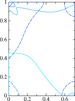
Fermi surfaces with Fermi velocity as a color weight

This section shows how to draw the Fermi surface, using color to delineate the Fermi velocity.

The first step is to make the Fermi velocities on a fine k mesh. Do this with the following:

lmf -vnk=51 ctrl.fe  --quit=band
lmdos fe -vnk=51 --dos~bands=3:6~rdm~window=-.05,.05~npts=101~mode=3  --kresm=-0.001939

lmdos finds all tetrahedra that encompass the Fermi level (which can be read from the output as -0.001939). and compute the DOS or related quantity at that energy. The --dos tage is explained here. mode=3 tells lmdos to generate not the DOS, but the velocity. This data is written to file dosq.h5, and can be read by lmf with the coldos flag as will be shown shortly.

lmdos should generate the following:

 <|v|> (spin 1) at Ef.  Avg 0.1807 a.u. = 0.1706 x 10^6 m/s.  Resolve by band:
  ib   <|v|>       ib   <|v|>       ib   <|v|>       ib   <|v|>
   3   0.5727  |    4   0.2197  |    5   0.0000  |    6   0.0000  |
 total DOS(Ef) = 1.844866
 q- and band- resolved   4 bands  132651 qp  ef=-0.001939  microcell vol 1.25643e-6

 <|v|> (spin 2) at Ef.  Avg 0.3133 a.u. = 0.2958 x 10^6 m/s.  Resolve by band:
  ib   <|v|>       ib   <|v|>       ib   <|v|>       ib   <|v|>
   3   0.1733  |    4   0.1511  |    5   0.3086  |    6   0.6908  |
 total DOS(Ef) = 3.810278

Minority (spin 1) bands register no velocities for bands 5 and 6, because they do not cross the Fermi level. The majority (spin 2) bands all have some presence at E_F and for simplicity we will draw the Fermi surface only for that spin.

With dosq.h5 in hand, regenerate bnds.fe, this time including DOS (actually velocity) as a color weight:

echo '.5 .5 0  0 1     35      0 0 1   0 1     51      0.00    2:6' > fs.fe
lmf -vnk=51 ctrl.fe  --quit=band --band:con:coldos:fn=fs

For simplicity, we will draw the Fermi surface only for spin 2 (the majority spin since the magnetic moment is negative).

The contour plot maker needs to know what colors to use, and files to find the weights. Extract spin 2 bands 2,3,4,5,6 into files 2, 3, 4, 5, 6, and corresponding weights into files w2, w3, w4, w5, w6:

set ef = `grep efermi= bnds.fe | head -1 | vextract . efermi`
set rf = "-r:open -qr bnds.fe -shft=-$ef"
set rfw = "-r:open -qr bnds.fe"
mcx [ 2:6 -qr $rfw ]  [ i=2:6 -qr $rf -w \{i} ]  [ i=2:6 -qr $rfw ] [ i=2:6 -qr $rfw -w w\{i} ] -show

Note that variable rfw causes mcx to read the next array from bnds.fe, while rf does the same but subtracts the Fermi level before writing.

Put the following box into file plot.fs2. It is a script for the fplot utility. For each of 3, 4, 5, 6 It reads files with that name to draw the lines, and correspoinding w3, w4, w5, w6 for the weights.

Copy the box below into file plot.fs2 and do

fplot -pr91 -f plot.fs2
open fplot.ps

fplot -frme 0,1/sqrt(2),0,1  -x 0,1/sqrt(2) -y 0,1 -tmx .1
   -lt 1,bold=4 -con~col=0,0,0~colwt=0,0,1~range=.1,.9~wtfn=w3 0 3
   -lt 1,bold=4 -con~col=0,1,0~colwt=0,0,1~range=.1,.9~wtfn=w4 0 4
   -lt 1,bold=4 -con~col=1,0,0~colwt=0,0,1~range=.1,.9~wtfn=w5 0 5
   -lt 1,bold=4 -con~col=1,0,0~colwt=0,0,1~range=.1,.9~wtfn=w6 0 6

The range 0.1…0.9 signifies that the color for a weight of 0.1 or less is assigned to col, while it gets assigned to colwt. for a weight of 0.9 or more. The color for any weight linearly interpolates between these two limits. The Fermi velocity varies by roughly and order of magnitude with k.

Click here to see the image.

The figure shows that the excursion in velocity is quite large — roughly an order of magnitude.

Fermi surfaces with orbital character as a color weight

This section shows how to draw the Fermi surface, using color to delineate the orbital character. Here we will use two colors: red to denote the Fe d t_2g and green the Fe d t_eg character.

The xy, yz and xz orbitals are the t_2g orbitals, which correspond to m=(−2,−1,+1) as can be seen from this table. The remaining two (x²−y² and 3z²−r²) are the e_g orbitals, which correspond to m=(0,+2).

Do the following:

lmf ctrl.fe --band~con~scol@atom=fe@l=2@m=-2,-1,1~scol2@atom=fe@l=2@m=0,2~fn=fs

With eigenvalues + two color weights; bnds.fe has 30 panels of points in all (5 bands × 2 spins × (1+2)) We need to extract eigenvalue blocks spin-2 bands 6-10, then t_2g weights for these bands (panels 16-20), then e_g weights (panels 26-30)

set ef = `grep efermi= bnds.fe | head -1 | vextract . efermi`
set rf = "-r:open -qr bnds.fe -shft=-$ef"
set rfw = "-r:open -qr bnds.fe"
mcx [ 2:6 -qr $rfw ]  [ i=2:6 -qr $rf -w \{i} ]  [ i=2:6 -qr $rfw ] [ i=2:6 -qr $rfw -w t2g\{i} ] [ i=2:6 -qr $rfw ] [ i=2:6 -qr $rfw -w eg\{i} ] -show

Copy the box below into file plot.fs3

fplot -frme 0,1/sqrt(2),0,1  -x 0,1/sqrt(2) -y 0,1 -tmx .1
   -lt 1,bold=4 -con~colwt=1,0,0~wtfn=t2g3~colw2=0,1,0~wtf2=eg3~ 0 3
   -lt 1,bold=4 -con~colwt=1,0,0~wtfn=t2g4~colw2=0,1,0~wtf2=eg4~ 0 4
   -lt 1,bold=4 -con~colwt=1,0,0~wtfn=t2g5~colw2=0,1,0~wtf2=eg5~ 0 5
   -lt 1,bold=4 -con~colwt=1,0,0~wtfn=t2g6~colw2=0,1,0~wtf2=eg6~ 0 6

and do

fplot -pr91 -f plot.fs3
open fplot.ps

Click here to see the image.

One contour changes continuously between t_2g and e_g; the ones at the top are mostly t_2g but towards the right acquire some non-d-character; the small pocket at the bottom right is a mix of t_2g and non-d.

Fermi surfaces with spin texture as a color weight

If spin orbit coupling is turned on, spin-up and spin-down become coupled and in general z is no longer the spin quantization axis. The spin orientation of a particular state is dependent on k, and its variation over the Brillouin zone is sometimes called spin texture.

lmf and lm both have the ability to make Fermi surfaces using color to help identify the spin texture; this section demonstrates how to accomplish it.

First, spin orbit coupling modifies the Fermi energy, so before proceeding with the Fermi surface you need to make a band pass with spin-orbit coupling on. The instruction below does this and writes E_F to to file wkp.fe without modifying rst.fe. When making the bnads for the Fermi surface E_F will be read from wkp.fe. In the same pass we can use --minmax to find which bands cross the Fermi level.

lmf ctrl.fe -vso=1 --rs=1,0 -vnit=1 --minmax

You should see a table similar to this:

 Lowest, highest evals by band, spin 1
-0.6031 -0.2377  |   18   0.7954  1.8231  |   35   3.5802  4.7029
-0.5739 -0.2157  |   19   1.3848  2.8901  |   36   3.5802  4.7427
-0.2421 -0.1668  |   20   1.4077  2.8908  |   37   4.2034  5.1770
-0.2366 -0.0993  |   21   1.5199  2.8916  |   38   4.2579  5.1981
-0.1657 -0.0120  |   22   1.5926  2.9145  |   39   4.4612  5.3936
-0.1204 -0.0104  |   23   2.1238  2.9145  |   40   4.4614  5.4374
-0.0721  0.0080  |   24   2.1508  2.9511  |   41   4.6669  5.6310
-0.0585  0.1641  |   25   2.5000  3.3909  |   42   4.6669  5.6311
-0.0417  0.1659  |   26   2.5602  3.3909  |   43   5.4826  7.3238
-0.0089  0.1845  |   27   2.6157  3.5063  |   44   5.4826  7.3238
 0.0373  0.6277  |   28   2.6928  3.5524  |   45   5.7411  8.0617
  ...

For the calculation run here, the output shows that the Fermi level is −0.002; thus four bands (7,8,9,10) cross E_F.

Now we are ready to make the bands for the contour plot. Do the following to generate spin texture weights from the d orbitals (see here for available options to --band)

echo '.5 .5 0  0 1     35      0 0 1   0 1     51      0.00    7:10' > fs.fe
lmf ctrl.fe -vso=1 --rs=1,0 -vnit=1 --band~con~scolst@atom=fe@l=2~fn=fs

The spin texture option generates four color weights: charge, and x-, y-, and z- components of the magnetization. Since bnds.fe contains information for four bands, the file has 20 panels of points in all (4 bands × (1+4)): 1 group for the bands + 4 groups for color weights.

We will use the contour mode of the fplot utility to draw the Fermi surface. The first four blocks of bnds.fe hold the eigenvalues for bands 7-10; the next four hold charge weights (not used), then the next twelve the weights for the three magnetization directions. fplot in the contour mode requires the raster of eigenvalues to be in separate files for each band, and also their associated color weights. Thus we need to extract eigenvalues for the first four blocks, skip the charge weights, and then extract weights for the x-, y-, and z- components of the magnetization. This will entail 16 files in all. Since Fe is barely noncollinear, we will scale the x and y weights by a factor of 100 to emphasize the canting.

set ef = `grep efermi= bnds.fe | head -1 | vextract . efermi`
set rf = "-r:open -qr bnds.fe -shft=-$ef"
set rfw = "-r:open -qr bnds.fe"
mcx [ i=7:10 -qr $rf -w \{i} ] [ i=7:10 -qr $rfw ]  [ i=7:10 -qr $rfw -abs -s100 -w x\{i} ] [ i=7:10 -qr $rfw -abs -s100 -w y\{i} ] [ i=7:10 -qr $rfw -abs -w z\{i} ] -show

mcx reads the first four blocks (energy bands 7-10) and writes them to files 7, 8, 9, 10; it reads the next four blocks and does nothing with them; it reads the next four blocks, takes the absolute value (the sign of the weight indicates whether the canting is along +x or −x, which we won’t use here) and scales by 100, and writes to files x7, x8, x9, x10. The same is done for the y and z weights. It also turns out that the canting is better seen for contours a little below E_F; the instructions below draw them at E_F − 0.05 Ry.

Copy the box below into file plot.fs4

fplot -frme 0,1/sqrt(2),0,1  -x 0,1/sqrt(2) -y 0,1 -tmx .1
   -lt 1,bold=4 -con~colwt=1,0,0~wtfn=x7~colw2=0,0,1~wtf2=y7~ -0.05 7
   -lt 1,bold=4 -con~colwt=1,0,0~wtfn=x8~colw2=0,0,1~wtf2=y8~ -0.05 8
   -lt 1,bold=4 -con~colwt=1,0,0~wtfn=x9~colw2=0,0,1~wtf2=y9~ -0.05 9
   -lt 1,bold=4 -con~colwt=1,0,0~wtfn=x10~colw2=0,0,1~wtf2=y10~ -0.05 10

and do

fplot -f plot.fs4
open fplot.ps

Click here to see the image.

The purple sections are projects onto an even combination of x and y (equal mixture of red + blue), indicating a canting along the 45 degree line.