Making the dynamical GW self energy
This tutorial is intended as a follow-on to the the QSGW tutorial for Fe, where the QSGW self-energy is made. Alternatively you can run this tutorial as a stand-alone by copying the needed files from the directory where your Questaal distribution sits, as explained in the tutorial.
An exact one-body description of the many-body Schrödinger equation requires a time-dependent, non-hermitian potential, called the self-energy . This is because independent-particle states that solve a one-body Schrödinger equation are no longer eigenstates in the many-body case. Nevertheless many-body descriptions are usually characterized in terms of a one-particle basis. The imaginary part of carries information about the inverse lifetime (the time for decay of a state to another state).
is nonlocal in both space and time. Nonlocality in time implies that depends on two time coordinates and ; however in equilibrium it depends only on the difference . Converting time to its Fourier (frequency) representation, depends only on a single frequency . Nonlocality in space implies that depends on two coordinates and . Translational invariance of a crystal implies that for translations between one unit cell and another, depends only on one (lattice) translation vector . With a Fourier from to representation, depends only on one vector. For points within a unit cell, depends on two coordinates and confined to a unit cell. Thus in general is written as .
Note: QSGW has two forms for the self-energy, the fully dynamical one, and the “quasiparticlized” form, which has a nonlocal but static self-energy derived from the dynamical . There is an editor for the quasiparticle form also, useful for other contexts. For applications of the static editor, see this page.
This tutorial shows how to use the GW machinery to construct and analyze a fully nonlocal . Questaal can generate , in many-body perturbation theory, using the GW machinery, which this tutorial covers. It can also make site local matrix elements of via Dynamical Mean Field Theory (DMFT). DMFT is a single-site approximation; it is nonlocal in time but nonlocal in space only between orbitals and on the same site. (Within the DMFT subspace, usually d orbitals in transition metals and f orbitals in f-shell elements, is nonlocal within those orbitals; in other words, the potential is orbital-dependent.) However the time-dependence in DMFT is calculated to a higher level of theory than is done for the GW approximation.
The main utility used to analyze a dynamical is lmfgws. The DMFT package generates in a different way but, once created, can also use lmfgws to analyze it.
Scattering from GW or DMFT originates from scattering between electrons : it corrects for some of the error inherent in a static one-body hamiltoan, that must be present when approximating the two-body potential in the Schroedinger equation.
Discorder can also create Other forms of scattering. Two kinds of disorder Questaal has facilities to manage those from lattice or spin disorder.
The Coherent Potential Approximation, or CPA replaces a true atom with some effective average atom (either alloys or atoms of one kind but different moment orientations) Even though it is a one-body approximation, the CPA construction implies that, like DMFT, is nonlocal in time but local in space. It operates as a stand-alone package.
Brillouin zone unfolding is designed to deal with lattice or spin disorder, like the CPA but done with supercells. lmfgws has the capability to analyze spectral functions that are derived from supercells but unfolded to the Brillouin zone of a smaller cell. (Here the scattering comes from Umklapp processes coupling states k’ with k, induced by disorder.)
This tutorial does the following:
- Generate the dynamical self-energy Σ(k,ω) using lmsig. For now it writes the self-energy to files SEComg.UP and SEComg.DN.
- Translate the files into a dynamical self-energy file se.fe that the dynamical self-energy postprocessor lmfgws can read. This is done with the spectral utility.
- The dynamical self-energy editor built into the postprocessor lmfgws, and is documented on this page.
Next follows applications of lmfgws to elemental iron, a bcc transition metal. The tutorial will show that the usual quasiparticle picture works reasonably well with roughly ±1 eV of the Fermi level, but quickly breaks down outside that range.
- Compute the the interacting density-of-states Fe and compare it to the independent-particle DOS
- Make the spectral function A(k,ω) near the H point, and also simulate photoemission spectra there.
- Compute the interacting joint density-of-states and imaginary part of the dielectric function from the interacting Green’s function.
- Make the interacting band structure along given symmetry lines, similar to what is reported in ARPES measurements.
The final section of the tutorial combines broadening of the spectral function from coulomb interactions (same as the preceding parts) with broadening from lattice or spin disorder. It is written to be completely independent of the other sections.
Table of Contents
- Table of Contents
- Preliminaries
- Theory
- The LQSGW Approximation
- Introduction
- Make the GW dynamical self-energy
- spectral, the self-energy translator
- Dynamical self-energy editor lmfgws
- Editor instructions
- Editor Application : Compare interacting and independent-particle density-of-states in Fe
- Editor Application : Spectral Function of Fe near the H point
- Editor Application : Interacting joint Density-of-States and Optics
- Editor Application : Interacting band structure
- Editor Application : Generating spectral functions from Brillouin zone unfolding of a supercell
- Getting started
- 1. Set up input files for 1-atom cell and establish the density is self-consistent
- 2. Construct a two atom supercell of Fe
- 3. Confirm that input conditions for the two-atom cell yield an approximately self-consistent density
- 4. Make GWinput and pqmap files for the supercell
- 5. Make dynamical self-energy for the supercell
- 6. Generate the supercell spectral function along symmetry lines
- 7. Generate the noninteracting band structure for the one-atom cell
- 8. Generate the noninteracting band structure for the two-atom cell
- 9. Make k-decomposed weights and QP bands in zone-unfolded supercell along symmetry lines
- 10. Make QP spectral function in the unfolded Brillouin zone
- 11. Interpolate supercell dynamical self-energy in points in syml.fe
- 12. Generate the BZ-unfolded dynamical spectral function on lines given in syml.fe
- References
Preliminaries
This tutorial assumes you have completed a QSGW calculation for Fe, following the QSGW Fe tutorial. Alternatively, you can treat this as a stand-alone tutorial. In that case you can starts from a fresh directory, and copy files from Questaal’s distribution to get started (complications can arise if you do not start from a fresh directory).
It also assumes the standard Questaal executables are in your path, e.g. lmf and lmgw.sh.
Theory
Z factor renormalization
Begin with a noninteracting Green’s function , defined through an hermitian, energy-independent exchange-correlation potential . refers to a particular QP state (pole of ). There is also an interacting Green’s function, .
The contribution to from QP state is
where is the pole of .
Write the contribution to from QP state as
Note that this equation is only true if is diagonal in the basis of noninteracting eigenstates. We will ignore the nondiagonal elements of . Note that if is constructed by QSGW, this is a very good approximation, since at . Approximate G by its coherent part:
where
defines the factor. The dependence of and on is suppressed.
Define the QP peak as the value of where the real part of the denominator vanishes.
and so
Note that in the QSGW case, the second term on the r.h.s. vanishes by construction: the noninteracting QP peak corresponds to the (broadened) pole of G. Thus the QSGW energy bands have a physical interpretation as excitation energies, and they coincide with the peaks in the spectral function of G.
The group velocity is . For the interacting case it reads
Use the ratio of noninteracting and interacting group velocities as a definition of the ratio of inverse masses. From the chain rule
Ignore the dependence of on . Write as , and use the definition of to get
So
In the QSGW case the quantity in parenthesis vanishes. Thus QSGW there is no “mass renormalization” from the ω-dependent self-energy, Σ(ω).
Coherent part of the spectral function
Write as
Rewrite as
Using the standard definition of the spectral function, e.g. Hedin 10.9:
the approximate spectral function is
which shows that the spectral weight of the coherent part is reduced by Z.
Simulation of Photoemission
(needs cleaning up)
Energy conservation : requires (see Marder, p735, Eq. 23.58)
where Eb is the binding energy and is the energy of the electron after being ejected. (Marder defines with the opposite sign, making it positive).
Momentum conservation : The final wave vector kf of the ejected electron must be equal to its initial wave vector, apart from shortening by a reciprocal lattice vector to keep kf in the first Brillouin zone.
Let be the energy on exiting the crystal, the work function and and are called the electron binding energy and “inner potential.”
Then
The total momentum inside the crystal, , is linked to the kinetic energy measured outside the crystal through Eq.(1). The kinetic energy is linked to the binding energy through the equation where is the work function of the analyzer. Usually . The Fermi level is defined such that . The inner potential is defined by scanning the range of photon energy under the constraint of normal emission: then the -point can be identified and by using Eq.(1), and the inner potential experimentally determined.
The momentum of the particle in free space is
Resolve into components parallel and perpendicular to the surface
After passing through the surface, is modified to ; this is what is actually measured.
The conservation condition requires
is conserved on passing through the surface; thus . is not conserved; therefore
The wave number shift is then
and the crystal momentum actually being probed by the experiment is
The LQSGW Approximation
Kutepov’s LQSGW theory of is a linearized form of QSGW. He constructs the quasiparticlized self-energy from a Taylor series around the origin. In his formalism (treating each band indpendently and suppressing band index, for simplicity of presentation) replaces the interacting
by omitting the second order and higher terms of an expansion in
simplifies to a linear function of
We use a bar to denote the factor since it is defined at :
Evidently is the eigenvalue of a hamiltonian defined as the one-body part of , but adding the static part of . The (linearized) energy-dependence of modifies this eigenvalue to read
is identical to the QSGW if is a linear function of .
Now let us retain the quadratic term and determine the shift in to estimate the difference between LQSGW and QSGW. Let us denote the LQSGW eigenvalue as . Expanding to second order we obtain, to lowest order in :
Introduction
The dynamical GW self-energy is made using the main GW script, lmgw.sh, which is assumed to be in your path together with the other binaries compiled in your build directory.
Steps in this tutorial are fast enough that you don’t need to execute in parallel, but you can do so. For the band code lmf and self-energy postprocessor lmfgws, preface the executable with MPI instructions suitable for your hardware, e.g. env MKL_NUM_THREADS=2 OMP_NUM_THREADS=2 mpirun -n 8 lmf. For the GW part the setup is more complicated. The user’s guide for lmgw.sh explains how the different parts of a GW calculation can be parallelized independently, but in this tutorial we assume a simple construct, typical when your executable uses the Intel MKL library.
Note: This tutorial is adopted from the standard test case $toplevel/gwd/test/test.gwd --mpi=#,# fe 5 .
Initial files
Note: If you are starting from the point where you completed the QSGW tutorial for Fe, you do not need to copy any files from the distribution, but you need to copy sigm.fe to sigm.in for the rest of the steps to work.
If starting from scratch, Copy the following setup files:
cp $toplevel/src/gwd/test/fe/{syml.fe,syml2.fe,fs.fe} $toplevel/src/gwd/test/fetb/{GWinput.gw,switches-for-lm,sigm.in,{basp,ctrl,site,rst}.fe} .
cp GWinput.gw GWinput
$toplevel is the directory where your Questaal distribution sits, e.g. ~/lm.
The QSGW static self-energy Σ0 was generated using the tight-binding form of the basis set, but this tutorial uses unscreened basis functions. Conversion requires two modifications.
- The self-energy Σ0 (in file sigm.in) must be rotated to an unscreened form.
- In this setup, file switches-for-lm controls whether the basis is screened or not. (This file as given contains –tbeh –v8 -vrsham=2 which turns on the screened basis.) lmgw.sh, passes the contents of switches-for-lm as command-line switches to various executables.
Make these modifications as follows:
lmf --tbeh --v8 -vrsham=2 fe --scrsig:ifl=sigm.in:ofl=sigm.fe:in=s:out=u
sed -i.bak 's/--tbeh --v8 -vrsham=2/--v8/' switches-for-lm
This step isn’t needed, but you can confirm that the setup generates a self-consistent density in the unscreened form
lmf `cat switches-for-lm` fe --quit=rho
You should see that the RMS change in the density is small, a few times 10−5.
Make the GW dynamical self-energy
This section makes the dynamical self-energy Σ(k,ω). Note only the diagonal matrix elements (in the eigenfunction basis) of Σ(k,ω) are calculated.
The instructions in this section should create SEComg.UP and SEComg.DN. These files contain Σ(k,ω), albeit in a not particularly readable format; they will be translated to an hdf5 format (se.h5) before postprocessing steps are performed.
Note: If self-consistency were entire, the input Σ0,in would match Σ0,out generated by the GW cycle. This is almost the case, not exactly so. The difference is slight but not totally negligible very near EF because lmsig makes Σ(k,ω), from the QP levels generated from Σ0,in, and calculates EF from them. Note also EF that lmsig uses Gaussian broadening with sampling to make Σ(k,ω), where as lmf uses tetrahedron integration. This is discussed further in the next section.
If you are starting from the QSGW Fe tutorial, clean the directory by removing these files
rm -rf meta mixm.fe mixsigma atom.h5 bz0.h5 bz.h5 dcs.h5 eigen.h5 evec.h5 moms.h5 ppbrdc.h5 ppbrd.h5 sig.h5 vcc.h5 vc.h5 w0.h5 0run
If you repeat this section, clean the directory by removing these files
rm -rf SEComg.{UP,DN} meta mixm.fe se se.h5 se2.h5 se.fe out.hsfp0 out.spectral out2.spectral out.lmfgws sigm sig.h5 sigma.fe spf.fe spf2.fe spf_qp_unf.fe spf_unf.fe bnds1.fe bnds2.fe bnds.h5
The dynamical self-energy maker needs some files generated by earlier steps in GW cycle, so they needed to be created first.
If you are running in parallel mode, make the pqmap file first, as the QSGW tutorial for Fe
lmfgwd ctrl.fe `cat switches-for-lm` --job=0 --lmqp~rdgwin --batch~np=4~pqmap@plot
Create the screened coulomb interaction needed for the self-energy
lmgw.sh --incount --stop=w0 --iter=1 --maxit=1 --sym --tol=1e-5 --split-w0 --mpirun-1 "env OMP_NUM_THREADS=2 MKL_NUM_THREADS=2 mpirun -n 1" --mpirun-n "env OMP_NUM_THREADS=2 MKL_NUM_THREADS=2 mpirun -n 4" ctrl.fe > out.lmgw
Note: The instruction uses OpenMP with 2 threads, and MPI with 4 processors (16 threads in all). You may need to adapt these switches. If you are running in serial mode, remove the mpirun portions all together. Parallelization isn’t important here: this step executes in a few seconds.
Make the dynamical self-energies SEComg.UP and SEComg.DN either in parallel or serial mode.
env OMP_NUM_THREADS=2 MKL_NUM_THREADS=2 mpirun -n 4 lmsig --v8 --rdwq0 --dynsig~nw=401~wmin=-2.0~wmax=2.0~bmax=11 ctrl.fe >& lsg
In parallel mode it should execute in about 10 minutes Macbook Pro with 8 cores. (The exact MPI instruction will depend on your hardware.) For serial mode, remove env OMP_NUM_THREADS=2 MKL_NUM_THREADS=2 mpirun -n 4.
Note: before proceeding to post-processing steps (Applications sections) be sure to convert the self-energies generated by lmsig into a format lmfgws can read; see documentation for the spectral utility.
Note: For reasons of cost, only the diagonal element of Σjj of Σij(k,ω) is calculated. Also for reasons of cost, Σjj is usually computed on a relatively coarse k and frequency mesh, and for a limited number of states. The preceding instruction uses an energy window of ±2 Ry, on an evenly spaced frequency mesh of 401 points, and computes Σjj for j=1·11. It uses a k mesh of 8×8×8 divisions (29 irreducible points). This is too coarse for detailed analysis, but lmfgws can interpolate both the k and frequency mesh, as explained briefly below, and demonstrated in the Applications parts of this tutorial.
The 1-shot GW self-energy maker, hsfp0, has a mode (--job=4) make the dynamical Σ(k,ω). Some changes to GWinput are needed. lmfgwd will automatically make these changes if you used switch --sigw in the QSGW tutorial.
With your text editor, modify GWinput. Change these two lines:
--- Specify qp and band indices at which to evaluate Sigma
into these four lines:
***** ---Specify the q and band indices for which we evaluate the omega dependence of self-energy ---
   0.01 2   (Ry) ! dwplot omegamaxin(optional)  : dwplot is mesh for plotting.
                  : this omegamaxin is range of plotting -omegamaxin to omegamaxin.
                  : If omegamaxin is too large or not exist, the omegarange of W by hx0fp0 is used.
Also change these lines
*** Sigma at all q -->1; to specify q -->0.  Second arg : up only -->1, otherwise 0
  0  0
to
*** Sigma at all q -->1; to specify q -->0.  Second arg : up only -->1, otherwise 0
  1  0
If you have removed intermediate files, you must remake them up to the point where the self-energy is made. Do:
$ lmgwsc --wt --sym --metal --tol=1e-5 --getsigp --stop=sig fe
This step is not necessary if you have completed the QSGW Fe tutorial without removing any files.
The next step will make Σ(kn,ω) on a uniform energy mesh −2 Ry < ω < 2 Ry, spaced by 0.01 Ry at irreducible points kn, for QP levels specified in GWinput. This is a fairly fine spacing so the calculation is somewhat expensive.
- Run hsfp0 (or better hsfp0_om) in a special mode --job=4 to make the dynamical self-energy.
export OMP_NUM_THREADS=8
export MPI_NUM_THREADS=8
$(dirname $(which lmgw))/code2/hsfp0_om --job=4 > out.hsfp0
Notes on the Fermi level and enforcement of the QSGW condition
The dynamical self-energy is computed as a function of frequency. To the extent the QSGW self-consistency condition is satisfied, that is Σ(k,ω=EQP-EF) = Σ(0)(k), the pole of the Green’s function is given solely by EQP for this condition to be properly satisfied.
However it may not be exactly satisfied, for example if the self-consistency is not fully realized, or for reasons noted earlier. In any case, the dynamical postprocessor lmfgws normally enforces this condition, unless you specify otherwise. Since the enforcement depends on knowledge of the quasiparticle EF, discrepancies will appear depending on how EF is chosen. Usually the uncertainty in EF is unimportant, but there is structure near EF on the scale of the uncertainty, which can make a difference. To work around this the lmfgws editor has instructions to allow you to specify it. The most automatic way is to tell it to find EF from a finely spaced k mesh (see getef in the instructions below). You can also specify EF by hand (see ef= in the instructions).
Once you specify EF, lmfgws will enforce the QSGW condition, unless to tell it not to.
Note : QP eigenvalues in SEComg.UP and SEComg.DN are written relative to the Fermi level, so they may be interpreted as a frequency. In the metallic case, the Fermi level is calculated from the noninteracting hamiltonian by gaussian smearing (see the output file lrdata4gw). In the insulating case, it takes the middle of the bandgap.
Notes on interpolating the self-energy in k and ω
As noted earlier, Σ(k,ω) is computed on relatively coarse k- and ω- meshes. However, quantities often need to be determined on a finer k-mesh, and also a finer ω-mesh. This is accomplished by an interpolation scheme: interpolation is reasonable because Σij(k,ω) varies smoothly with both k and ω.
Normally when Σjj(k,ω) to a k where it is not known, both the dynamical self energy and the one-particle QP levels are interpolated to the target point, by linear interpolation from closest-neighbor k points where it is known.
Note : at present the interpolating algorithm relies on Σ being supplied on a uniformly spaced mesh of points. lmfgws will not operate when interpolation is needed and Σ is not on a uniform mesh.
k-interpolation is usually less accurate than ω-interpolation, because the former is typically kept to a coarse mesh for reasons of cost. While interpolating Σ(k,ω) is necessary, interpolating the one-particle levels is not, because lmfgws can readily generate them for any k. This can be used to avoid interpolation for the QP levels, and improve it for Σ(ktarg,ω) For the latter, it can be accomplished by adding a frequency shift to Σ(ktarg,ω) that corresponds to the difference between the interpolated QP level and the explicitly calculated one.
spectral, the self-energy translator
spectral is a utility that reads SEComg.UP (and SEComg.DN in the spin polarized case). SEComg.UP and SEComg.DN contain the diagonal matrix element for each QP level j, for each irreducible point kn in the Brillouin zone, on a regular mesh of points ω as specified in the previous section. If the absence of interactions, so the spectral function would be proportional to δ(ω−ω*), where ω* is the QP level (see Theory section).
Interactions give an imaginary part which broadens out the level, and in general, shifts and renormalizes the quasiparticle weight by Z. As noted in the Theory section, there is no shift if is the QSGW self-energy ; there remains, however, a reduction in the quasiparticle weight. This will be apparent when comparing the interacting and noninteracting DOS.
Most often, spectral is use to translate SEComg.UP (SEComg.DN) into file se.ext (or h5 file se.h5) which the dynamical self-energy postprocessor lmfgws can read. This is discussed in the below.
spectral also has a limited ability to create spectral functions in its own right, as described next. However this capability is now subsumed in lmfgws, and it is recommended that you use spectral only to generate an se file suitable for lmfgws.
Unfortunately SEComg.UP (SEComg.DN) do not contain information about the Fermi level which lmfgws will need to align QP levels it calculates with those in these files. You can extract it from the output of the GW cycle as follows
efsigm=`grep 'Fermi level for sigma' lw0 | awk '{print $9}'`  [bash]
set efsigm = `grep 'Fermi level for sigma' lw0 | awk '{print $9}'`  [tcsh]
To run spectral, do one of the following
spectral --pr31 --ws --nw=1 --efry=$efsigm > out.spectral; mv se se.fe
spectral --pr31 --wsh --nw=1 --efry=$efsigm > out.spectral
The first (with --ws) writes an ASCII file and renames it to se.fe; ths second (with --wsh) writes the same information in hdf5 format, se.h5. lmfgws can read either format; this tutorial uses the hdf5 format.
At this point the self-energy is ready for the self-energy postprocessor lmfgws. You can use spectral directly to generate spectral functions (next section), but it is largely a legacy code and lmfgws is much more versatile. It works in an editor mode: instructions for its use are shown below.
Use spectral to directly generate spectral functions for q=0
Note: This documents legacy functionality in spectral. It has a limited ability to directly generate spectral functions from raw output SEComg.{UP,DN} which this section demonstrates.
Do the following:
spectral --eps=.005 --domg=0.003 '--cnst:iq==1&eqp>-10&eqp<30'
Command-line arguments are described here. In this context they have the following meaning:
--eps=.005 : 0.005 eV is added to the imaginary part of the self-energy. This is needed because as ω→0, ImΣ→0. Peaks in A(k,ω) become infinitely sharp for QP levels near the Fermi level.
--domg=.003 : interpolates Σ(kn,ω) to a finer frequency mesh. ω is spaced by 0.003 eV. The finer mesh is necessary because Σ varies smoothly with ω, while A will be sharply peaked around QP levels.
--cnst:expr : acts as a constraint to exclude entries in SEComg.{UP,DN} for which expr is zero.
expr is an integer expression using standard Questaal syntax for algebraic expressions. It can that can include the following variables:- ib (band index)
- iq (k-point index)
- qx,qy,qz,q (components of q, and amplitude)
- eqp (quasiparticle energy, in eV)
- spin (1 or 2)
The expression in this example, iq==1&eqp>-10&eqp<30, does the following:
generates spectral functions only for the first k point (the first k point is the Γ point)
eliminates states below the bottom of the Fe s band (i.e. shallow core levels included in the valence through local orbital)
eliminates states 30 eV or more above the Fermi level.
spectral writes files sec_ibj_iqn.up and sec_ibj_iqn.dn which contain information about Im G for band j and the k point kn. A sec files takes the following format:
# ib=   5  iq=   1  Eqp=   -0.797925  q=   0.000000   0.000000   0.000000
#     omega         omega-Eqp     Re sigm-vxc    Im sigm-vxc      int A(w)      int A0(w)       A(w)           A0(w)
  -0.2721160D+02 -0.2641368D+02 -0.6629516D+01  0.1519810D+02  0.2350291D-04  0.6897219D-08  0.7774444D-02  0.2281456D-05
  -0.2720858D+02 -0.2641065D+02 -0.6629812D+01  0.1520157D+02  0.4701215D-04  0.1379602D-07  0.7776496D-02  0.2281979D-05
  ...
spectral also makes the k-integrated DOS. However, the k mesh is rather coarse and a better DOS can be made with lmfgws. See below.
 spectral: read 29 qp from QIBZ
 Dimensions from file(s) SEComg.(UP,DN):
 nq=1  nband=9  nsp=2  omega interval (-27.2116,27.2116) eV with (-200,200) points
 Energy mesh spacing = 136.1 meV ... interpolate to target spacing 3 meV.  Broadening = 5 meV
 Spectral functions starting from band 1, spin 1, for 9 QPs

          file            Eqp      int A(G)   int A(G0) rat[G] rat[G0]
      sec_ib1_iq1.up   -8.743948     0.8473     0.9999     T     T
      sec_ib2_iq1.up   -1.674888     0.8251     0.9999     T     T
      sec_ib3_iq1.up   -1.674819     0.8251     0.9999     T     T
 ...
 writing q-integrated dos to file dos.up ...
 Spectral functions starting from band 1, spin 2, for 9 QPs

          file            Eqp      int A(G)   int A(G0) rat[G] rat[G0]
      sec_ib1_iq1.dn   -8.458229     0.8447     0.9998     T     T
      sec_ib2_iq1.dn    0.015703     0.8718     0.9999     T     T
      sec_ib3_iq1.dn    0.016072     0.8700     0.9999     T     T
...
 writing q-integrated dos to file dos.dn ...
Dynamical self-energy editor lmfgws
This section explains the features lmfgws has to construct various properties of the interacting Green’s function. Later sections will demonstrate some of these features for Fe.
lmfgws is the dynamical self-energy editor, which performs a variety of postprocessing of the GW or DMFT self-energy for different purposes. Typically is supplied on a uniform mesh of points . It can interpolate in both and to provide information for any and .
lmf computes properties the noninteracting QSGW band structure, while lmfgws computes the corresponding interacting one. They require the same input files; in addition lmfgws requires the dynamical self-energy, se.ext or se.h5, which is explained in an earlier part of the tutorial for the GW context.
Given se.ext or se.h5, lmfgws can:
- Generate the spectral function at specified points
- compute the interacting density-of-states (DOS). Entails an integral of over .
- Simulate ARPES with a simple model for final-state scattering (not shown in this tutorial)
- Compute the noninteracting and interacting joint density-of-states and imaginary part of the dielectric function from the interacting Green’s function
- Generate the interacting band structure along specified symmetry lines, which can be compared to what is commonly reported in ARPES experiments.
- Generate the interacting Fermi surface (not very informative in the present QSGW context, but quite useful in a non Fermi liquid context, which DMFT can supply; see e.g. this paper).
Note 1: It is not required that the given kn are supplied on a regular mesh, but in such a case some instructions of the editor (those that require k interpolation) are not allowed. Also in that a case you must tell the editor that you are not using a uniform mesh (see irrmesh in the instructions below).
Note 2: In Feb. 2022, lmfgws was parallelized to work with MPI. (If use the editor with MPI, typically you need to operate strictly in batch mode as well.) Most of the editor instructions have been parallelized, though not all of them. Run lmfgws as mpirun -np # lmfgws ...
These files will be made in later stages of this tutorial. If you have already run parts of this tutorial, delete these files:
rm -f sdos.fe seia.fe pes2.fe pesqp0.fe spq.fe spq-bnds.fe seq.fe jdos-lmf.fe jdosni.fe
Generate se.fe using the spectral utility
Use spectral to translate SEComg.UP (and SEComg.DN since this system is magnetic) into se.fe:
spectral --pr31 --ws --nw=1 > out2.spectral
cp se se.fe
- --ws tells spectral to write the self-energy to file se for all k points, in a special format designed for lmfgws. Individual files are not written. It must be renamed to se.ext for use by lmfgws.
- --nw=1 tells spectral to write the self-energy on the frequency mesh it was generated; no frequency interpolation takes place. This will be done by lmfgws.
Editor instructions
This sections documents the instruction set of the dynamical self-energy editor. Codes that can generate the input for this editor are spectral and lmfdmft.
Invoking the editor: interactive vs batch mode
You can run the editor interactively, or in batch mode.
- Interactive mode
- To operate lmfgws in interactive mode, invoke
lmfgws ctrl.fe `cat switches-for-lm` --sfunedYou should see:
 Welcome to the spectral function file editor.  Enter '?' to see options.

 Option :
The editor operates interactively. It reads a command from standard input, executes the command, and returns to the Option prompt waiting for another instruction.
The editor will print a short summary of instructions if you type ? <RET> .
- Batch mode
- You can also run the editor in batch mode by stringing instructions together separated by a delimiter, e.g.
lmfgws fe '--sfuned~units=eV~eps@.01'The delimiter ( ~ in this case), is the first character following --sfuned. lmfgws will parse through all the commands sequentially until it encounters “quit” instruction ( ~q ) which causes it to exit. If no such instruction is encountered, lmfgws returns to the interactive mode.
Instruction set
Note: Other delimiters may be used in place of @ assumed below, but if you are operating the editor in batch mode, be sure to distinguish this delimiter from the batch mode delimiter. You can use a space as a delimiter here, but in batch mode, you need to enclose ‘--sfuned’ in single quotation marks. If you run lmfgws with mpirun, it may be safer to avoid using spaces, as mpirun may strip the quotes.
readsek[flags] | readsekb[flags] | readsekh[flags]
reads the self-energy from an ASCII file (readsek), binary file (readsekb), or hdf5 file (readsekh). In the absence fn, the file name defaults to se.ext for the ASCII case, seb.ext for the binary case, and se.h5 for the hdf5 case. Data is read in the basis of 1-particle eigenfunctions for whatever states are supplied in the file. When reading a file generated by the QSGW cycle it typically reads header information, including number of spins in file; number of bands and k points; number of frequencies and the smallest and largest values; the list of bands stored in the file (a subset of all the bands may be stored); and the stored chemical potential if it is written into the file.The se file structure is documented on this page for both ASCII and hdf5 formats.
Some points of note:
Data is stored for a collection of k points; the list of points is written in the file. These points may, or may not constitute a uniform mesh of points.
QP levels are stored relative to the chemical potential (which may, but need not, be written in the header).
Only the diagonal elements of the potentials are read. The full complement of static potentials consist of the static QSGW self-energy , the Fock exchange , and ,
The se file may, but need not, contain these potentials. se files generated lmfdmft or in the Brillouin zone unfolding mode of lmf contain only Σ(k,ω). On the other hand se files generated by the current GW implementation typically contain: (1) the k-points where Σ is stored; (2) the QP levels generated from the starting self-energy Σ0,in; (3) the quasiparticlized self-energy Σ(0); (4) the dynamical self-energy Σ(k,ω).
For the GW-generated case, after reading the file it checks how well the QSGW condition is satisfied at self-consistency, namely that Σ(k,ω) should equal Σ(0)(k) at the QP level. The result is written to stdout in a line like this one:
<(sig-vxc)@eQP>=-0.000004 RMS=0.000074 shift=-0.000948 RMS=0.029138 Adjust=F Optional flags are strung together and separated by a delimiter, taken as the first character. The sequences below assume the delimiter is @ .\
- @fn=nam use nam for self-energy file name [for readeb and readebr the file should be a bands file in h5 format].
- @useef writes the file chemical potential into the Fermi level.
- @irrmesh points are not on a regular k mesh : no k interpolations allowed
- @ib=list after reading data from file, pare bands read from file to those in list
- @minmax print minimum and maximum QP levels for each band
- @dc=# subtract double counting from Re sigma(omega) after reading, mode # (for DMFT)
- @scl=# scale Σ(k,ω) and Σ(0)(k) by #.
- @makeqpse Not documented yet
readeb[flags] | readebr[flags]
readeb and readebr are instructions for the Brillouin zone unfolding mode. The scattering has a different origin from the coulomb scattering generated by the dynamical self-energy (loss of k as a good quantum number). Thus its generation and usage proceed a bit differently, and information is read from a bands file, written in hdf5 format (see here for documentation). It has many features in common with the readse instructions, and share the same optional flags. readeb and readebr are equivalent to each other except the weight (see Eq. (5) in this tutorial) is read as written for readeb, while for readebr the weight is turned into .
units@Ry | units@eV
Select Rydberg units or electron volt units (default=Ry).
Note: the se file can store data in either eV or Ry units; lmfgws internally converts it to whatever units you select.getef[@n=#1[#2,#3]@show] | getef=#1[,#2,#3]
Finds the QSGW fermi level for a specified mesh #1[#2,#3], and sets it as the default to be used in future operations. If no mesh is specified the mesh taken from se.ext is used.
Optional show causes lmfgws to suppress assigning the calculated EF to the default value.evsync[@frzsig]
Replaces quasiparticle levels EQP read from se.ext by recalculating them internally with lmf, shifting the energy zero to EF.
If EF has already been supplied externally (typically by readsek@useef, ef=#, or getef), that value is used. Otherwise it uses the internal EF found when EQP are generated.After synchronizing EQP, the QSGW condition is imposed : Σ(k,ω)=Σ(0)(k) = 0 at EQP. For QSGW, it is imposed by shifting Σ(0)(k) for QSGW generated se.ext. Optional argument frzsig causes lmfgws not to show how well the QSGW condition is imposed, but not to update the self-energy.
eps val
add a constant val to Im Σ, needed to broaden spectral functions so that integrations are tractable.ef=# | ef0=#
Assign #@useef to the Fermi level, overriding the internally calculated value.
Note: the order in which you use this switch is important. If you use the ef switch before readsek, QP levels are shifted by μ−Ef when they are subsequently read (provided the chemical potential μ is supplied in the se file). If you use this switch after readsek, no shifts are added. In such a case you likely want to realign the QP levels with evsync after readsek. Always enter # in Ry units.
Use ef0=# to set the QP Fermi level. In QSGW it is not distinct from ef, but it is in DMFT.
- dos|jdos|imeps [getev=#1,#2,#3] | [nq=#1,#2,#3] ib=list wts=strn [getev|getev[=#1,#2,#3]] [nw=#|domg=#] [range=#1,#2] [isp=#]
dos integrates the spectral function to make both the QP and spectrum DOS (writes to sdos.ext or sdos2.ext).
jdos integrates either the QP or interacting spectral function to make the joint DOS (writes to jdos.ext).
imeps integrates either the QP or interacting spectral function to make Im ε (writes to opt.ext or optni.ext).
Options are:- ib=lst restrict contribution to spectra from QP states in list.
- nq=#1,#2,#3 Evaluate the physical quantity on a specified mesh. This entails interpolating Σj(kn,ω) to a new uniform mesh of k points, defined by (#1,#2,#3) divisions. Use between 1 and 3 numbers.
- getev Calculate the QP levels on the supplied mesh, and enforce the QSGW condition. The enforcement should have already been satisfied if evsync was invoked previously and the Fermi level is consistent with the mesh.
- getev=#1,#2,#3 Calculate the QP levels on a specified mesh, and enforce the QSGW condition. Thus it is similar to nq=#1,#2,#3 except the QP part (i.e. QSGW part) of the hamiltonian need not be interpolated and the QSGW condition for Σj(kn,ω) is enforced.
- wts=strn (Applies to dos only) Add extra columns to file sdos, writing projections of dos onto a subspace, defined through the orbitals of the basis set.
The projection uses a Mulliken population analysis of the orbitals comprising the basis, to resolve a normalized eigenfunction into some portion of it.
This is the same procedure used to make color weights for energy bands and it uses the same “color weights” syntax as the--bandswitch uses.
Example:wts#scol@atom=u#scol2@atom=co#scol3@atom=ge
will generate a pair of columns each for three decompositions: orbitals belonging to U, Co, and Ge respectively.
If the crystal has nothing but U, Co, and Ge, the sum of the three partial dos should add to unity.
Hazard: wts requires two levels of delimiters ( @ and # in the example above).
Take care that these delimiters are distinct from the delimiter separating arguments to dos,
as well as the one separating batch commands if you are using batch mode. - nw=n Refine the given energy mesh by interpolating Σ to an n multiple of the given energy mesh. n must be an integer.
- range=#1,#2 Generate DOS in a specified energy window (#1,#2), in eV.
- kT Temperature, units of omega (applies only to jdos and imeps).
- a0 Spectra for noninteracting spectral function (only for jdos and imeps).
- isp=# Generate DOS for spin # (1 or 2). Default value is 1.
- se iq=n | q=#1,#2,#3 | allq | band[@args] ib=list | ibx=list [getev[=#1,#2,#3]] [a2qp] [nw=n|domg=#] [isp=#] [range=#1,#2]
Make Σ(ω) and A(ω) for given q and range of bands.
Specify which q by:- iq=n index to qn, from list in QIBZ. Writes to seia.ext, or to seia2.ext for second spin.
- q=#1,#2,#3 q-point in units of 2π/alat. lmfgws will interpolate Σ(qn) to any q. Writes to seia.ext.
- allq Σ(ω) is made for all q in the irreducible bz and written to seq.ext.
- band A(ω), Σ(ω) are made for qp along symmetry lines and written to spq.ext.
Use this mode to draw interacting energy bands, in conjunction with plbnds −sp
Optional @args are parsed like options of the --band switch.
Other arguments: - ib=list Sum together Aj(ω) derived from QP states j in list.
- ibx=list ibx and ib perform the same function, but ibx writes out more information, e.g. Aj(ω) is resolved by band, writing each Aj(ω) in succession.
- getev Do not interpolate QP energy but calculate it at each q where Σ and A are to be evaluated.
- getev=#1,#2,#3 Generate evals on independent mesh with #1,#2,#3 divisions of uniformly spaced points. EQP may have to be interpolated if the mesh does not contain q.
- a2qp Extract the QP energy from the peak in and write it for the one-particle energy when writing spq.ext.
- nw=n Refine the given energy mesh by interpolating Σ to an n multiple of the given energy mesh. n must be an integer.
- range=#1,#2 Generate spectral function in a specified energy window (#1,#2).
- wx=# Interpolate Σ(ω) and A(ω) to frequency # and write to disk only data for this frequency (for Fermi surfaces).
- pe | peqp iq=n | q=#1,#2,#3 ib=# [getev[=#1,#2,#3]] [nw=# | domg=#] [nqf=#] [ke0=#] [isp=i] [range=#1,#2]
Model ARPES for given q and band(s). Writes to pes.ext or pes2.ext.
pe uses the spectrum self-energy, while peqp uses just the quasiparticle hamiltonian. Final-state effects are folded into both. Only the latter works with SO coupling now.
Required arguments are:- iq=n index to qn, from list in QIBZ. Alternatively specify q by:
- q=#1,#2,#3 q-point in units of 2π/alat. lmfgws will interpolate Σ(qn) to any q.
- ib=list Sum together PE spectrum derived from QP states j in list. See here for the syntax of integer lists.
Options are: - getev Do not interpolate energy but calculate it at q.
- getev=#1,#2,#3 Generate evals on independent mesh with #1,#2,#3 divisions of uniformly spaced points.
- nw=n Refine the given energy mesh by interpolating Σ to an n multiple of the given energy mesh. n must be an integer.
- isp=i Generate spectra for spin i (1 or 2). Default value is 1.
- nqf=n number of mesh points for final state integration. Default is 200.
- ke0=# kinetic energy of emitted electron. KE+V0=ℏω−φs+V0
- range=#1,#2 Generate spectral function in a specified energy window (#1,#2)
qsgwh
Generates the Quasiparticle “self-energy” (in practice the QP levels relative to the Fermi level, treated as δ-functions in energy)savesea [fn]
saves spectrum DOS or self-energy + spectral function, in ASCII format. In the absence fn, the file name defaults to seia.ext or seia2.ext when writing band and k-resolved spectral functions (se or pe) and to sdos.ext or sdos2.ext when writing spectrum dos (dos).savese [fn]
saves q-interpolated self-energy + spectral function in binary format. In the absence fn, the file name defaults to seib.ext.- q
quits the editor unless information has generated that has not been saved. Program terminates. - a
(abort) unconditionally quits the editor. Program terminates.
Editor Application : Compare interacting and independent-particle density-of-states in Fe
This section shows how to generate the interacting density-of-states with lmfgws. The interacting and non-interacting density-of-states are compared. To obtain a reasonably well converged interacting density-of-states it is necessary to interpolate Σ(kn,ω) to a finer k- and ω- mesh.
Once you have created the self-energy file, run lmfgws in batch mode:
env OMP_NUM_THREADS=4 MKL_NUM_THREADS=4 mpirun -n 4 lmfgws fe `cat switches-for-lm` '--sfuned~units eV~readsekh~eps .030~dos isp=1 range=-10,10 nq=32 nw=30~savesea~q'
This invocation writes the spectral and noninteracting DOS to file sdos.fe. The mesh is very fine, so the interpolation takes a little while (maybe a minute). You can use MPI, as shown in the instruction above, to speed up the calculation.
To run in serial mode, remove the env OMP_NUM_THREADS=4 MKL_NUM_THREADS=4 mpirun -n 4 .
lmfgws should generate output similar to the following:
 Entering the spectral function file editor.  Parsing command-line options ...

 Option : units eV
 Units set to eV
It is convenient to generate quantities in eV, rather than atomic Rydberg units.
 Option : readsekh
 Data from file se.h5:  nq=29  nband=11  nsp,nspx=2,2  freq (-27.211386,27.211386) eV (401 points). Ef = 0.02847 Ry = 0.387356 eV
 file q-points match standard mesh? ... yes
 QSGW condition for 29 pts  <(sig-vxc)>@eQP=-0.000002 RMS=0.000015  shift <dw>=-0.000175 RMS=0.11648  Adjust=F
The self-energy is read and a check is made on the QSGW condition.
 Option : eps .030
 Smearing set to 0.03 eV
The noninteracting DOS needs an imaginary part to smooth out the δ-functions
 Option : dos isp=1 range=-10,10 nq=32 nw=30

 Interpolate to 32x32x32 k mesh
 Make QSGW energy bands on 32x32x32 k mesh
 evalqp: Get  k-mesh ...
 BZMESH: 897 irreducible QP from 32768 ( 32 32 32 )  shift= F F F
 TETIRR: sorting 196608 tetrahedra ... 39615 inequivalent ones found

 SUGWS:  interpolate self-energies, 11 band(s), 897 qp, spin 1
 mean eval shift (897 qp, 11 bands) = 0.000000
 DOS on  (32,32,32) qp mesh  energy window (-9.9956,9.9956), 4409 points (spacing=0.0045)  eps=0.03

 ... End loop over q: sumcheck ag0 1581200
Make the spectrum DOS for spin 1, in the energy range (-10,10) eV, interpolating Σ to a k mesh 32×32×32 divisions, and refining the energy mesh by a factor of 30. The as-given k mesh is 8×8×8 divisions.
 Option : savesea
 wrote data to ascii file sdos
Write the DOS to file sdos.fe
 Option : q
 Exit 0 exit sigfun editor
 CPU time:  11.860s   Wall clock 11.875s  at  13:28:34 02.01.2025  on  ellery
Exit the editor.
You can compare the interacting and noninteracting dos by comparing columns 2 and 3. You can also compare the dos generated by lmf. It should align with the noninteracting DOS computed here, but lmf uses tetrahedron integration to make the DOS (more accurate than the sampling integration used here). So comparing the two is a good check of the quality of the k-integration.
You can make the QP DOS yourself, but to speed things up just copy an already generated DOS from the build directory to your working directory.
cp $toplevel/src/gwd/test/fe/dosp.fe dosp.fe
The following script draws a figure comparing the DOS generated the three different ways, using the fplot utility. Cut and paste the contents of the box below into script file plot.dos.
% char0 ltdos="1,bold=3,col=0,0,0"
% var ymax=1.4 dy=0.4 dw=.00 ymax+=dy emin=-10 emax=5 ef=0
fplot

% var ymax-=dy+dw dy=0.4 dmin=0 dmax=3
 -frme 0,1,{ymax-dy},{ymax} -p0 -x {emin},{emax} -y {dmin},{dmax} -tmy 1 -1p
 -colsy 3 -lt 1,bold=3,col=.5,.5,.5 sdos.fe
 -colsy 2 -lt {ltdos} -ord y -qr dosp.fe
 -colsy 2 -lt 1,bold=3,col=1,0,0 sdos.fe
 -lt 2,bold=3,col=0,0,0,2,.5,.05,.5 -tp 2~{ef},{dmin},{ef},{dmax}
Draw the figure with
$ fplot -f plot.dos
$ open fplot.ps   [choose your postscript file viewer]

Notes on the figure :
- The black line (col=0,0,0) is the noninteracting DOS generated by lmf.
- The grey line (col=.5,.5,.5) is the noninteracting DOS A0(ω), generated by lmfgws.
- The red line (col=1,0,0) is the interacting DOS A(ω), generated by lmfgws
- Grey and black lines nearly coincide, as they should if the DOS is well converged. Note that the black line was generated from energy bands with the tetrahedron method, the other effectively by integrating G0(k,ω) by sampling with a smearing of 30 meV.
- The noninteracting DOS at the Fermi level is D(EF)≅1/eV (one spin). The Stoner criterion for the onset of ferromagnetism is I×D(EF)>1, where I is the Stoner parameter, which DFT predicts to be approximately 1 eV for 3d transition metals. Combining DOS for the two spins would indicate that the Stoner criterion is well satisfied.
- The interacting DOS is smoothed out, and is roughly half the amplitude of the noninteracting DOS. This is also expected: the Z factor for the d states is about 0.5.
Editor Application : Spectral Function of Fe near the H point
This example computes the self-energy for a q point near (1,1,0) — the H point. It is calculated from band 2 for the majority spin and bands 2,3 for the minority spin. These bands were chosen because of their proximity to the Fermi level. The first line generates A(ω) for spin 1, the second for spin 2
lmfgws fe `cat switches-for-lm` '--sfuned~units=eV~eps@.01~readsekh~evsync~se@q=1.05,2.91,1.01@ib=5@nw=10@getev=12@isp=1~savesea~q'
lmfgws fe `cat switches-for-lm` '--sfuned~units=eV~eps .01~readsekh~evsync~se q=1.05,2.91,1.01 ib=5,6 nw=10 getev=12 isp=2~savesea~q'
The first command writes a file seia.fe, the second seia2.fe. To interpret the command-line argument, refer to the editor manual.
The following makes a picture comparing A (solid lines) and A0 (dashed lines), majority spin (black) and minority spin (red)
fplot -x -9,5 -y 0,1 -colsy 2 -lt 1,col=0,0,0 seia.fe -colsy 3 -lt 2,col=0,0,0 seia.fe -colsy 2 -lt 1,col=1,0,0 seia2.fe -colsy 3 -lt 2,col=1,0,0 seia2.fe
open fplot.ps   [choose your postscript file viewer]

The QP at −4 eV is already very broad, showing that the QP picture becomes an increasingly poorer approximation as the energy becomes more remote from the Fermi energy.
You should see a weak plasmon peak in the majority spin band near −8 eV.
Editor Application : Interacting joint Density-of-States and Optics
lmfgws can make the joint density-of-states (JDOS) and the macroscopic dielectric function. The joint DOS is given by
Note that is a (weak) function of temperature since the Fermi function contains temperature.
In the limit of noninteracting particles and this expression reduces to the standard expression for joint density-of-states
The following computes joint DOS (noninteracting case) using the lmf optics package. It renames the file for future comparison.
env OMP_NUM_THREADS=4 MKL_NUM_THREADS=4 mpirun -n 4 lmf -vnkabc=32 fe `cat switches-for-lm` -vlteto=0 -voptmod=-1 --quit=rho
cp jdos.fe jdos-lmf.fe
The following computes joint DOS for both static and interacting QS_GW_ self-energies, using lmfgws.
env OMP_NUM_THREADS=4 MKL_NUM_THREADS=4 mpirun -n 4 lmfgws fe `cat switches-for-lm` '--sfuned~units@eV~readsekh~eps@.040~jdos@range=-10,10@nq=32@a0@nw=5~savesea~q'
env OMP_NUM_THREADS=4 MKL_NUM_THREADS=4 mpirun -n 4 lmfgws fe `cat switches-for-lm` '--sfuned~units@eV~readsekh~eps@.040~jdos@range=-10,10@nq=32@nw=5~savesea~q'
The first command makes file jdosni.fe, the second jdos.fe.
The following will make a postscript file, with frequency on the abscissa in eV:
fplot -frme 0,.7,0,.5 -x 0,10 -ab 'x1*13.6' -colsy 2,3 -ord y/13.6 jdos-lmf.fe -lt 2,col=1,0,0 -colsy 2,3 jdosni.fe -lt 3,bold=5,col=0,1,0 -colsy 2,3 jdos.fe

Black (joint DOS computed by lmf) and Red (noninteracting joint DOS by lmfgws) are very similar. Dotted green is the corresponding joint DOS with the dynamical self-energy. There is a strong reduction of order because of loss of quasiparticle weight in the coherent part of
Optics are very similar the joint DOS. In the absence of a vertex, is proportional to the joint DOS, decorated by the matrix elements of velocity operator, . The latter is usually calculated in terms of the momentum operator . In Ry units reads
The following makes using lmf with gaussian sampling integration.
env OMP_NUM_THREADS=4 MKL_NUM_THREADS=4 mpirun -n 4 lmf -vnkabc=32 fe `cat switches-for-lm` -vmefac=2 -vlteto=0 -voptmod=1 --quit=rho
cp opt.fe opt-lmf.fe
The following computes for both static and interacting QSGW self-energies, using lmfgws.
env OMP_NUM_THREADS=4 MKL_NUM_THREADS=4 mpirun -n 4 lmf -vnkabc=32 fe `cat switches-for-lm` -vlteto=0 -voptmod=1 -vmefac=2 --quit=rho --opt:woptmc
env OMP_NUM_THREADS=4 MKL_NUM_THREADS=4 mpirun -n 4 lmfgws fe `cat switches-for-lm` '--sfuned~units@eV~readsekh~eps@.040~imeps@range=-10,10@nq=32@a0@nw=5~savesea~q'
env OMP_NUM_THREADS=4 MKL_NUM_THREADS=4 mpirun -n 4 lmfgws fe `cat switches-for-lm` '--sfuned~units@eV~readsekh~eps@.040~imeps@range=-10,10@nq=32@nw=5~savesea~q'
In the first step lmf generates and stores matrix elements of the velocity operator in file optdatac.fe for lmfgws. The latter commands generate optni.fe and opt.fe. They are calculated in the same way as in the independent particle case, but for spectral functions from the static and interacting QSGW self-energies.
Draw a picture of the three independent calculations of Im ε:
fplot -x 0,10 -frme 0,.7,0,.5 -frmt th=3,1,1 -xl "~{w} (eV)" -x 0,10 -y 0,35 -ab 'x1*13.6' -colsy 2,5 opt-lmf.fe -lt 2,col=1,0,0 -colsy 2,5 optni.fe -lt 3,bold=5,col=0,1,0 -colsy 2,5 opt.fe

Note that lmf uses Ry units; we specified eV in the lmfgws instruction. Thus when comparing Im ε, the abscissa for opt-lmf.fe is scaled to eV.
You should see something similar to the figure shown on the right. For all three data, contributions are resolved into majority and minority parts. The physically relevant Im ε is the sum of the two.
Black (Im ε computed by lmf) and Red: (Im ε computed by lmfgws, noninteracting case) are very similar. Dotted green is the corresponding Im ε computed in the RPA with the dynamical self-energy. There is a strong reduction in intensity because of loss of quasiparticle weight in the coherent part of .
Editor Application : Interacting band structure
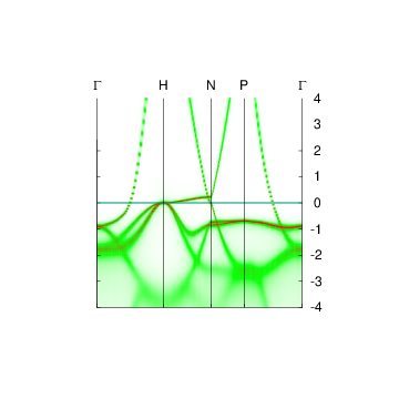
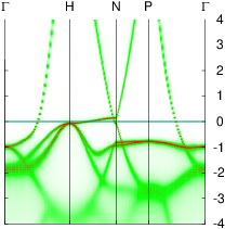
This application uses lmfgws to generates the band structure of the interacting Green’s function, i.e. the k-resolved spectral function along symmetry lines similar to a band plot for a noninteracting . Peaks in the spectral function correspond to the band structure; the plot can be compared directly to the bands of the noninteracting G0. Use syml.fe from that tutorial, or use file syml2.fe, which contain the symmetry lines as appear in Figure 1 of this Phys. Rev. B paper. Invoke lmfgws in batch mode as follows:
env OMP_NUM_THREADS=4 MKL_NUM_THREADS=4 mpirun -n 4 lmfgws fe '--sfuned~units eV~readsekh~eps .01~evsync~se band:fn=syml ib=4:11 nw=10 getev=12 isp=1 range=-10,10'
The self-energy editor carries out the following (see editor instructions) for more detail:
- units eV
Set units to eV - readsek
Read se.fe - eps .01
Add 10 meV smearing to Im Σ - evsync
refresh quasiparticle levels read from se.fe by recalculating them. - se band:fn=syml ib=4:11 nw=10 getev=12 isp=1 range=-10,10
Generate the self-energy and spectral function along symmetry lines given in file syml.fe. Include bands 4-11, and generate on a frequency mesh 10× finer than the one in se.h5. getev refines the k-mesh to a 12×12×12 mesh, and using that mesh to interpolate bands along symmetry lines in syml.fe. Generate bands for spin 1 in an energy window [−10,10] eV.
lmfgws writes a file, spq.fe.
Invoke plbnds in “spectral function mode:”
plbnds -sp~atop=10~window=-4,4~drawqp spq.fe
It will generate a gnuplot script file gnu.plt together with a data file spf.fe.
Run gnuplot
gnuplot gnu.plt
open spf.ps   [choose your postscript file viewer]
to generate and view postscript file spf.ps.
The yellow line is the QP band structure from the noninteracting QSGW self-energy. By construction it falls at the peak of the interacting band structure. Blue shows the interacting band structure. Broadening goes to zero at the Fermi level (as it should, according to Fermi liquid theory), but is already quite large below 2 eV. In the conduction band, broadening stays small because the bands are of highly dispersive sp character and the high kinetic energy makes them less immune to scattering. For d states in the valence band the broadening increases much more rapidly.
Note : overlaying the QP bands (yellow) shows the QSGW condition is well satisfied, but it obscures the heat map changing from green (low intensity) to red (high intensity). Try running plbnds without the drawqp modifier. You should see a picture like the one shown.
Editor Application : Generating spectral functions from Brillouin zone unfolding of a supercell
Note: This section is independent of the preceding parts of the tutorial. It shows how scattering from the dynamical self-energy with and scattering from lattice disorder can be combined. If you want to look at the effect from disorder alone (leaving out the many-body scattering), see the Additional exercises portion of Brillouin zone unfolding tutorial.
A one-particle hamiltonian yields sharply defined energy levels (becoming bands in an infinite system). However it is only an approximation to the true hamiltonian, because the electron-electron interaction is two-body and cannot be cast exactly into a one-particle form. (For a particularly lucid analysis, see Richard Martin’s book1.) The difference between the true and one-particle hamiltonian may be thought of as a scattering potential; this is the basis for Landau’s quasiparticle theory, and in order to be valied the scattering cannot be too strong. The QSGW prescription may be thought of as a means to generate a nearly optimal one-particle hamiltonian.
Lattice and spin disorder (imagining spins as local moments attached to magnetic sites and their random rotation against each other) are another source of scattering. The latter can be modeled by supercells (with disorder included) and decomposing the eigenstate into different k vectors of the original cell. The redistribution of QP weight among multiple k is how disorder is modeled in Questaal. In practice it is accomplished with the Brillouin zone unfolding scheme.
Coulomb, and lattice and spin disorder act together. This section of the tutorial provides the steps needed to combine coulomb disorder (any many body effect) with lattice and/or spin disorder (a one-body effect). The latter are not actually present in this tutorial because we take an oversimplified case. We use a 2-atom supercell of Fe, without disorder. Thus the decomposition of an eigenstate into different k components is trivial: each state maps fully onto only one of the possible distribution of states. It does show BZ unfolding will show how the spectral function of an artificial 2-atom supercell aligns with that of the one-atom cell. If disorder were added, points of distinct k in the small cell would couple and be a source of disorder.
Note: This tutorial is adopted from the standard test case $toplevel/gwd/test/test.gwd --mpi=#,# fe 7, and all the steps explained here are carried out in that check.
Getting started
This part of the tutorial requires a QSGW density and self-energy for the one-atom cell, and a corresponding one for the two-atom cell. For the former we will copy files essentially in the same was as the preceding section; only here we use the tight-binding form for the hamiltonian. The 1- and 2- atom cells will share some files in common. The files that need to be different for the two cases are:
- site file, assigned to site.fe and site2.fe respectively for the 1-atom and 2-atom cases.
- restart file, assigned to rst.fe and rsta.fe respectively
- QSGW static self-energy Σ(0)(k), assigned to sigm.fe and sigma.fe respectively
- A file passed as command line arguments to executables like lmfgws, assigned to switches-for-lm0 and switches-for-lm, respectively.
Note that rsta.fe and sigma.fe are standard restart and Σ(0)(k) files, but written in ASCII format.
Combining two kinds of disorder is a bit complicated, so the tutorial requires many steps to proceed. To get started, create a fresh directory and copy the files as in the preceding parts of the tutorial:
cp $toplevel/src/gwd/test/fe/{syml.fe,syml2.fe,fs.fe,pqmap-2} $toplevel/src/gwd/test/fetb/{GWinput.gw,switches-for-lm,sigm.in,{basp,ctrl,site,rst}.fe} .
After the input files are copied, this tutorial proceeds with the following steps:
Confirm that the (rst.fe,sigm.fe) pair generates a self-consistent density. This step is not essential but serves as a sanity check (stdout = out.lmf1)
- Construct a two atom supercell of Fe (stdout = out.lmscell)
- make site2.fe
- make rsta.fe
- make sigma.fe
- make switches-for-lm
Confirm that the rsta.fe,sigma.fe pair yields and approximately self-consistent density for the supercell. This step is not essential but serves as a sanity check (stdout = out.lmf2)
Make GWinput and pqmap for the supercell (out.lmfgwd). GWinput is needed to generate the self-energy; the latter is not required but allows the self-energy make to run faster on a multicore machine.
Make dynamical self-energy Σ(k,ω) for the supercell for all k points in the irreducible Brillouin zone of the supercell, writing it to se.h5 (stdout = out.lmgw, lsg)
Generate the spectral function for the supercell along symmetry lines syml.fe, making files gnu.spf2.plt, spf2.fe (stdout = out.scell.lmfgws)
Generate the QP band structure for small cell, writing to bnds1.fe. This is not required but it forms a useful point of comparison with the interacting band structure (stdout = out.1.lmf)
Generate the QP band structure for supercell, writing to bnds2.fe. Also not required but it forms a useful point of comparison with the interacting band structure (stdout = out.2.lmf)
Make k-decomposed weights and QP bands in zone-unfolded supercell along symmetry lines in syml.fe, written to bnds.h5 (stdout = out.unf.lmf)
Make QP spectral function in the unfolded Brillouin zone along the lines in syml.fe, generating gnu.spf1.plt and spf_qp_unf.fe (stdout = out.unf.QP.lmfgws). This step is exactly analogous to the Brillouin zone unfolding tutorial.
Interpolate dynamical self-energy in supercell to points in file syml.fe, writing se2.h5 (stdout = out.2atom.unf.lmfgws)
- Generate the BZ-unfolded dynamical spectral function along lines in syml.fe, writing files gnu.spf_unf.plt and spf_unf.fe (stdout = out.2atom.unf.lmfgws)
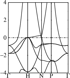
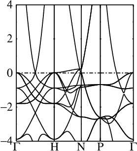
In these steps energy bands and spectral functions will be created that should like the six panels shown below.
The top three panels will be referred to as (a), (b), (c) and correspond to the noninteracting band structures of steps 7, 8, and 9.
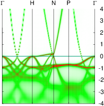
The bottom three panels will be referred to as (d), (e), (f) and correspond to the spectral functions (aka interacting band structures) of the one-atom cell developed in a previous section, and those generated steps 6,and 12, respectively. In the 2-atom cell, spectral functions at the Γ and H points are the same.


1. Set up input files for 1-atom cell and establish the density is self-consistent
Move initial files to proper locations and run lmf
cp sigm.in sigm
ln -s -f sigm sigm.fe
cp switches-for-lm switches-for-lm0
lmf `cat switches-for-lm0` fe --quit=rho > out.lmf1
Confirm it is nearly self-consistent:
grep DQ out.lmf1
You should see that the RMS change in the output density is on the order of 10−5.
2. Construct a two atom supercell of Fe
The simple cubic lattice holds two bcc sites. Construct the site file with the supercell maker
lmscell ctrl.fe `cat switches-for-lm0` --plx~1,0,0,0,1,0,0,0,1 --wsite~shorten=0~map~short~fn=site2 --tfix~shorten=0 > out.lmscell
Confirm that site2.fe contains a simple cubic lattice with 2 Fe atoms in the cell.
Create switches-for-lm for the supercell. In bash:
sw="-vfile=2 --rs=2,2 --rsig:ascii -vnkabc=12 -vnkgw=6 -vamix=t -vbeta=.3 `cat switches-for-lm`"
echo $sw > switches-for-lm
or tcsh
set sw = "-vfile=2 --rs=2,2 --rsig:ascii -vnkabc=12 -vnkgw=6 -vamix=t -vbeta=.3 `cat switches-for-lm`"
echo $sw > switches-for-lm
Use the static self-energy editor to make Σ0 for the supercell from the one atom cell, and the restart file editor to make a restart file for the supercell.
lmf ctrl.fe --shorten=no  `cat switches-for-lm0` '--wsig~edit~scell sigq nq=6,6,6 outfile=sigm site2' >> out.lmscell
lmf ctrl.fe --shorten=no `cat switches-for-lm0` --rsedit~rs~scell@outfilea=rsta@site2  >> out.lmscell
lmf ctrl.fe --rsig --shorten=no  `cat switches-for-lm` --wsig~ascii >> out.lmscell
cp sigm.in sigm.fe
Note that the number of k divisions is reduced to 6 from 8, as the Brillouin zone is smaller.
The last line restores Σ0 for the one atom cell, as it was overwritten in the 2-atom construction.
3. Confirm that input conditions for the two-atom cell yield an approximately self-consistent density
rm -f mixm.fe
lmf `cat switches-for-lm` fe --quit=rho > out.lmf2
grep DQ out.lmf2
The RMS DQ should be about 10−4 — slightly larger than the one-atom cell. This is to be expected since k mesh is different. The Fermi surface integrations are slightly inexact especially because Fe is a metal.
4. Make GWinput and pqmap files for the supercell
Make GWinput and pqmap for the supercell, assuming you will use 4 processors. (You do not need pqmap; that step is optional.)
lmfgwd ctrl.fe `cat switches-for-lm` -vsig=0 --job=-1 --classicGWinput > out.lmfgwd
lmfgwd ctrl.fe `cat switches-for-lm` -vsig=0 -vnit=1 --rs=1,0 --job=0 --lmqp~rdgwin --batch~np=4~nodes=1~pqmap@plot@fill=.80 >> out.lmfgwd
As the test case contains a residual of a legacy code, GWinput is made where some inputs are put directly in it (--classicGWinput).
--——————-
Upon completion of step 4 all the necessary input files are prepared for both the one-atom and two-atom cases, including those needed to make the dynamical self-energy
5. Make dynamical self-energy for the supercell
This part is essentially identical to the generation of the dynamical self-energy documented for the one-atom cell except it is for the two-atom cell. Besides the number of atoms being different, the k mesh is different as well.
Here we use 16 cores, split into 4 OpenMP threads and 4 MPI processes.
lmsig will make the dynamical self-energy, but it needs some files prepared by prior steps to run. These are made with the following
lmgw.sh --incount --stop=w0 --iter=1 --maxit=1 --sym --tol=1e-5 --split-w0 --mpirun-1 "env OMP_NUM_THREADS=4 MKL_NUM_THREADS=4 mpirun -n 1" --mpirun-n "env OMP_NUM_THREADS=4 MKL_NUM_THREADS=4 mpirun -n 4" ctrl.fe > out.lmgw
Now you can generate the dynamical self energy for the supercell
env OMP_NUM_THREADS=4 MKL_NUM_THREADS=4 mpirun -n 4 lmsig `cat switches-for-lm` --rdwq0 --dynsig~nw=401~wmin=-2.0~wmax=2.0~bmin=7~bmax=22 ctrl.fe >& lsg
It takes about 6 minutes on a standard desktop with 16 cores.
Translate the self-energy into an hdf5 file se.h5
efsigm=`grep 'Fermi level for sigma' lw0 | awk '{print $9}'`  [bash]
set efsigm = `grep 'Fermi level for sigma' lw0 | awk '{print $9}'`  [tcsh]
spectral --pr31 --wsh --nw=1 --efry=$efsigm > out.scell.spectral
As before, the Fermi level needs to be extracted and passed to spectral, as it is not supplied in SEComg.UP or SEComg.DN.
6. Generate the supercell spectral function along symmetry lines
This step parallels the generation of the interacting band structure for the one atom cell, except is done for the two atom supercell. The spectral function should look the same except that twice as many peaks appear because the Brillouin zone is folded.
Execution proceeds similarly to the one-atom cell developed earlier
env OMP_NUM_THREADS=4 MKL_NUM_THREADS=4 mpirun -n 4 lmfgws fe `cat switches-for-lm` '--sfuned~units=eV~readsekh~eps@.01~getef=6~evsync~se@band:fn=syml@ib=7:22@nw=10@getev=12@isp=1@range=-4,4' > out.scell.lmfgws
plbnds -sp~atop=10~window=-4,4 spq.fe >> out.scell.lmfgws
cp spf.fe spf2.fe
cat gnu.plt | sed s/spf.fe/spf2.fe/ > gnu.spf2.plt
except that now there are twice as many bands, ranging from 7-22 instead of 4-11. The last two steps copy gnu.plt to gnu.spf2.plt, and spf.fe to spf2.fe, to make way for spectral functions to be made later.
gnuplot gnu.spf2.plt; gs spf.ps
open spf.ps   [choose your postscript file viewer]
The figure should look essentially like the spectral function of the one-atom cell except that now there are twice as many bands folded in from other points in the Brillouin zone. In particular the Γ and H points become equivalent. Your figure should look like panel (e) above.
7. Generate the noninteracting band structure for the one-atom cell
This step performs a conventional band calculation for the one-atom cell
env OMP_NUM_THREADS=4 MKL_NUM_THREADS=4 mpirun -n  4 lmf ctrl.fe --shorten=no  `cat switches-for-lm0` --quit=rho > out.1.lmf
env OMP_NUM_THREADS=4 MKL_NUM_THREADS=4 mpirun -n  4 lmf ctrl.fe --shorten=no  `cat switches-for-lm0` --quit=rho --band:long:lbl=GHNPG:fn=syml >> out.1.lmf
cp bnds.fe bnds1.fe
The first lmf instruction is needed to get the Fermi level. The second makes bnds.fe, which is copied to bnds1.fe. Generate a figure for the band structure with
plbnds -spin1 -range=-4,4 -fplot~scl=.6,.7~ts=1 -ef=0 -scl=13.6 -lt=1,col=0,0,0,colw=.9,.9,.9 -lbl bnds1.fe; fplot -f plot.plbnds
open fplot.ps  [choose your postscript file viewer]
This is the standard spin-1 QSGW band structure of Fe (see panel (a) above).
8. Generate the noninteracting band structure for the two-atom cell
This step performs a conventional band calculation for the two-atom cell. It is the same as the preceding step, except for the two atom cell
env OMP_NUM_THREADS=4 MKL_NUM_THREADS=4 mpirun -n 4 lmf ctrl.fe --shorten=no `cat switches-for-lm` --quit=rho > out.2.lmf
env OMP_NUM_THREADS=4 MKL_NUM_THREADS=4 mpirun -n 4 lmf ctrl.fe --shorten=no `cat switches-for-lm` --quit=rho --band:long:lbl=GHNPG:fn=syml >> out.2.lmf
cp bnds.fe bnds2.fe
Generate a figure for the band structure with
plbnds -spin1 -range=-4,4 -fplot~scl=.6,.7~ts=1 -ef=0 -scl=13.6 -lt=1,col=0,0,0,colw=.9,.9,.9 -lbl bnds2.fe; fplot -f plot.plbnds
open fplot.ps  [choose your postscript file viewer]
This is the same spin-1 QSGW band structure for Fe, but in an artificially doubled cell (see panel (b) above).
9. Make k-decomposed weights and QP bands in zone-unfolded supercell along symmetry lines
This instruction parallels the first step of the Brillouin zone unfolding tutorial. It generates a bnds file like in step 8, but also computes the weights for resolving the band into two distinct k.
Because the cell is doubled, the Brillouin zone is folded in half. This instruction
h5dump -d q0sup bz0.h5
shows that k vectors (0,0,0) and (1,1,1) are equivalent in the supercell (these are the Γ and H points), while they are distinct in the one atom cell. Thus in the supercell k of the small cell is no longer a good quantum number, but is distributed across two distinct values.
In this step, each eigenstate is resolved into two weights which sum to one, and provide information about the distribution of the eigenstate into one of the k.
env OMP_NUM_THREADS=4 MKL_NUM_THREADS=4 mpirun -n 4 lmf --scell~job=-1~evrnge=7:22 ctrl.fe `cat switches-for-lm` --band~fn=syml > out.unf.lmf
env OMP_NUM_THREADS=4 MKL_NUM_THREADS=4 mpirun -n 4 lmf --scell~job=11~getef ctrl.fe `cat switches-for-lm0` --band~fn=syml~h5~lbl=GHNPG >> out.unf.lmf
The first instruction performs the decomposition of each eigenstate and writes the necessary information to evec.h5.
The second reads this information and writes the weights together with the QP levels to bnds.h5.
We can make a “quasiparticle spectral function”, meaning that the ordinary QP bands are reduced by the weight from the k decomposition. The weight is stored as data element colwt and has a function similar to color weights used to project bands onto orbitals. In this simple case there is no disorder so each weight is 0 or 1 (unless a band has an equivalent at the counterpart k point, in which case it the weight can be distributed between both).
Draw the bands weighted with the spectral weight as follows
plbnds -spin1 -range=-4,4 --h5 -fplot~scl=.6,.7~ts=1 -ef=0 -scl=13.6 -dat=unf -lt=1,col=0,0,0,colw=.9,.9,.9 -lbl bnds.h5 > out.plbnds
fplot -f plot.plbnds
You should see the bands belonging to the one-atom cell in bold, and the extra bands that arise from zone folding appear as light gray. Your figure should look like panel (c) above.
10. Make QP spectral function in the unfolded Brillouin zone
The information in step 9 can be presented another way, namely as a spectral function. lmfgws has a branch that treats the states of the supercell as states of the small cell with reduced weight. This yields a spectrum of broadened QP levels when disorder is present. It is more useful when there is real disorder, but we carry out the steps here to demonstrate how to carry it out.
env OMP_NUM_THREADS=4 MKL_NUM_THREADS=4 mpirun -n 4 lmfgws ctrl.fe `cat switches-for-lm0` '--sfuned~units@eV~readebr@fn=bnds@useef@irrmesh~eps=0.02~se^band@lbl=GHNPG@fn=syml^nomg=5001^range=-6,6' > out.unf.QP.lmfgws
env OMP_NUM_THREADS=4 MKL_NUM_THREADS=4 mpirun -n 1 plbnds -sp~atop=10~window=-4,4 spq.fe >> out.unf.QP.lmfgws
plbnds -sp~atop=10~window=-4,4 spq.fe >> out.unf.QP.lmfgws
cp spf.fe spf_qp_unf.fe
cat gnu.plt | sed s/spf.fe/spf_qp_unf.fe/ > gnu.spf1.plt
lmfgws makes a spectral function file spq.fe exactly analogous to the file generated from the dynamical self-energy. The last two steps rename the files to keep them distinct from other spectral functions.
You can draw a spectral function
gnuplot gnu.spf1.plt
open spf.ps  [choose your postscript file viewer]
Note : this step is exactly parallel to exercise 2 in the Brillouin zone unfolding tutorial.
11. Interpolate supercell dynamical self-energy in points in syml.fe
This is a preparatory step for the ultimate purpose of this section, namely to combine scattering from disorder with scattering from the electron-electron interaction. It is necessary because the self-energy is generated for the k mesh of the supercell, whereas for the BZ unfolding we need it on the points in syml.fe. Σ(k,ω) cannot be interpolated when working in small unit cell while reading Σ(k,ω) from the large one, so it is necessary to work in the supercell and interpolate Σ to the points of interest (those contained in syml.fe.) lmfgws has a special branch that interpolate Σ(k,ω) to a given set of points and writing the result to a new se file. Do the following
env OMP_NUM_THREADS=4 MKL_NUM_THREADS=4 mpirun -n 4 lmfgws fe `cat switches-for-lm` '--sfuned~units=eV~readsekh~se@intrp:ds=bnds.h5/qp@getev' > out.2atom.unf.lmfgws
The points must be supplied as a data set in an hdf5 file (in this case they are read from qp in bnds.h5). Once interpolated lmfgws writes a new self-energy file, se2.h5.
12. Generate the BZ-unfolded dynamical spectral function on lines given in syml.fe
We are finally ready to combine the BZ weights with the dynamical self-energy. It proceeds in a manner analogous to the section that made the interacting band structure in the one-atom cell; but there are differences. The self-energy is read from se2.h5 and readsekh is replaced with readsekh+readebr . This launches a special branch in lmfgws that reads the weights from bnds.h5 and scales each spectral function by the weight generated in step 9.
env OMP_NUM_THREADS=4 MKL_NUM_THREADS=4 mpirun -n 4 lmfgws fe `cat switches-for-lm0` '--sfuned~units=eV~readsekh+readebr@fn=se2~eps@.01~se@band:fn=syml@ib=7:22@nw=10@isp=1@range=-4,4' >> out.2atom.unf.lmfgws
Make a postscript file for the spectral function
plbnds -sp~atop=10~window=-4,4 spq.fe >> out.2atom.unf.lmfgws
cp spf.fe spf_unf.fe
cat gnu.plt | sed s/spf.fe/spf_unf.fe/ > gnu.spf_unf.plt
It writes files gnu.spf_unf.plt and spf_unf.fe.
Draw a figure with
gnuplot gnu.spf_unf.plt; gs spf.ps
open spf.ps   [choose your postscript file viewer]
Your figure should look like panel (f) above, and it is essentially identical to panel (d), obtained by a circuitous route. The same techniques can be used to study disordered systems. See for example, exercise 2 in the Brillouin zone unfolding tutorial, which presented a demonstration of spin disorder (without including scattering from coulomb interactions).
References
1 R. M. Martin, Electronic Structure, Cambridge University Press (2004).