Brillouin Zone Folding

This tutorial demonstrates how to unfold the band structure of a supercell onto a primitive cell.

What Brillouin zone unfolding does, a sketch

Suppose you construct an N-fold supercell of some primitive cell, meaning the lattice vectors of the supercell are integer multiples of the lattice vectors of the primitive cell, and the supercell volume is N times larger.

Bloch’s theorem tells us that k is a good quantum number, thus an eigenfunction of the periodic solid can be labeled with quantum numbers ${n\mathbf{k}}$.

Now consider two unit cells: a fundamental cell with lattice vectors $\mathbf{P}$ and a supercell with lattice vectors $\tilde{\mathbf{P}}$ concatenated from $N$ small cells, so that $\tilde{\mathbf{P}}{\mathbf{P}}^{-1}$ is an integer matrix. Then the Brillouin zone of the small cell is folded into the supercell so that $N$ k-points in the small cell $\mathbf{k}_1,...,\mathbf{k}_N$, become reciprocal lattice vectors $\tilde\mathbf{G}_1,...,\tilde\mathbf{G}_N$, of the large one. (The reciprocal lattice vectors of the fundamental- and super- cells are denoted by $\mathbf{G}$ and $\tilde\mathbf{G}$, respectively.) In the supercell k remains a good quantum number, albeit in an N-fold smaller Brillouin zone. We express eigenfunctions as linear combination of Bloch waves. Denote the Bloch waves of the supercell as $\tilde\chi^{\mathbf{k}}_{\tilde\mu}$, and the eigenfunctions as $\tilde\Psi^{n\mathbf{k}}$, while the same quantities without the tilde denote the analogous functions in the small cell.

Eigenfunctions are expanded as linear combinations of basis functions. For the large and small cells we have $$\tilde\Psi^{n\mathbf{k}}(\mathbf{r}) = \sum\nolimits_{\tilde\mu} \tilde{z}^{n\mathbf{k}}_{\tilde\mu} \tilde\chi^{\mathbf{k}}_{\tilde\mu}(\mathbf{r}) \qquad\qquad\qquad (1)$$ $$\Psi^{n\mathbf{k}}(\mathbf{r}) = \sum\nolimits_{\mu} {z}^{n\mathbf{k}}_{\mu} \chi^{\mathbf{k}}_{\mu}(\mathbf{r}) \qquad\qquad\qquad (2)$$

In Questaal, $\tilde\mu$ or $\mu$ becomes the compound indices ${\varepsilon}\mathbf{R}L$; in a plane wave basis $e^{i(\mathbf{k}{+}\mathbf{G}){\cdot}\mathbf{r}}$ they are the lattice vectors $\tilde\mathbf{G}$ or $\mathbf{G}$.

$\tilde\Psi$ can similarly be expressed as linear combinations of the basis functions $\chi_\mu$ of the small cell. The eigenvector is no longer diagonal in k, but it is diagonal in the family $\mathbf{k}{+}\mathbf{k}_i$. Then $$\tilde\Psi^{n\mathbf{k}}(\mathbf{r}) = \sum\nolimits_{\mu,i} \hat{z}^{n(\mathbf{k}+\mathbf{k}_i)}_{\mu} \chi^{\mathbf{k}+\mathbf{k}_i}_{\mu}(\mathbf{r}) \qquad\qquad\qquad (3)$$

One of the $\mathbf{k}_1,...,\mathbf{k}_N$ must be zero, and we will choose $\mathbf{k}_1=0$ by convention.

If in the supercell, every multiple or replica of the central cell has the same potential (an artificial N-fold duplication of the primitive cell), k of the primitive cell is a good quantum number, and the connection between $\hat{z}$ and $z$ is trivial: $\hat{z}^{n(\mathbf{k}+\mathbf{k}_i)}_{\mu} = {z}^{n\mathbf{k}}_{\mu} \delta_{\mathbf{k},\mathbf{k}_1}$ .

On the other hand if every multiple of the cell are similar but not identical, e.g. if phonons or spin disorder are included, they act as a perturbation relative to some average. Then ${z}^{n(\mathbf{k}+\mathbf{k}_i)}_{\mu}$ are not zero but small compared to ${z}^{n(\mathbf{k}+\mathbf{k}_1)}_{\mu}$. Thus the ratio $\hat{z}^{n(\mathbf{k}+\mathbf{k}_i)}_{\mu}/\hat{z}^{n(\mathbf{k}+\mathbf{k}_1)}_{\mu}$ should be not too different from 1 for $i{=}1$ and small for $i{>}1$. It is a measure of what is known as the Umklapp process when disorder originates from phonons, and in general a measure of scattering or disorder. It is of course not a requirement that the perturbation be small, but the interpretation of the supercell in the BZ of the primitive cell is no longer very meaningful.

It remains to determine the relative magnitudes of the $\hat{z}^{n(\mathbf{k}+\mathbf{k}_i)}_{\mu}$. In a plane-wave basis, this identification is simple, because the basis functions for the primitive and supercells are identical because the families $\{\mathbf{G}{+}\mathbf{k}_i\}$ and $\{\tilde\mathbf{G}\}$ are the same. Write Eqns (1) and (3) as $\sum\nolimits_{\tilde\mathbf{G}} \tilde{C}^n_{\mathbf{k}{+}\tilde\mathbf{G}} e^{i(\mathbf{k}{+}\tilde{\mathbf{G}}){\cdot}\mathbf{r}}$ and $\sum\nolimits_{\mathbf{G}{+}\mathbf{k}_i} C^n_{\mathbf{k}{+}\mathbf{G}{+}\mathbf{k}_i} e^{i(\mathbf{k}{+}\mathbf{G}{+}\mathbf{k}_i){\cdot}\mathbf{r}}$. Since for each ${\tilde\mathbf{G}}$ there is some $\mathbf{k}_i$ for which ${\mathbf{G}{+}\mathbf{k}_i}{=}{\tilde\mathbf{G}}$, Eqns (1) and (3) imply $\tilde{C}^n_{\mathbf{k}{+}\tilde\mathbf{G}} = {C}^n_{\mathbf{k}{+}\mathbf{G}{+}\mathbf{k}_i}$.

Noting that the eigenvector is normalized $$\sum_{\mathbf{k}_i} \sum_{\mathbf{G}} \left| C^{n}_{(\mathbf{k}+{\mathbf{G}}+{\mathbf{k}_i})}\right|^2 = 1 , \qquad\qquad\qquad (4)$$

the remaining QP weight after scattering from ${\mathbf{k}_1}$ to ${\mathbf{k}_{i>1}}$ can be expressed as the unscattered portion $$w_{n\mathbf{k}} = \sum_{\mathbf{G}} \left| C^{n}_{(\mathbf{k}+{\mathbf{G}})}\right|^2 \qquad\qquad\qquad (5)$$

Note that $w_{n\mathbf{k}}$ is a weight between 0 and 1 can for postprocessing purposes can be treated in the same way as weights from other ways to decompose an eigenstate, e.g. in a Mulliken decomposition of a eigenstate.

In practice, $w_{n\mathbf{k}}$ is calculated by dividing the $\tilde{C}^n_{\mathbf{k}{+}\tilde\mathbf{G}}$ into those for which correspond to some ${C}^n_{\mathbf{k}{+}\mathbf{G}}$ and the rest.

In general (this includes the Questaal basis), the $\{\chi^{\mathbf{k}+\mathbf{k}_i}_{\mu}\}$ and the $\{\tilde\chi^{\mathbf{k}}_{\tilde\mu}\}$ do not span an identical hilbert space. The $w_{n\mathbf{k}}$ can only determined approximately, e.g. by finding the $\hat{z}^{n(\mathbf{k}+\mathbf{k}_i)}_{\mu}$ that minimize the difference between Eqns (1) and (3). It is straightforward to do this formally, but in practice not so simple in Questaal, owing to the augmented-wave nature of the basis set. Moreover the procedure is time consuming when unfolding larger cells. Instead, the BZ unfolding implementation in Questaal currently determines $w_{n\mathbf{k}}$ essentially by Eq. (5). Since the envelope parts of the basis functions have a plane wave expansion, the envelopes are expanded in plane waves and $w_{n\mathbf{k}}$ determined from the interstitial part according to Eq. (5). This is not quite correct, since the proper eigenfunction has augmentation parts whose change on entering the supercell will not shift exactly in concert with the interstitial parts. This contribution is ignored.

Casting the supercell potential as a potential of the small cell with a Self-Energy

A noninteracting hamiltonian has a quasiparticle at every eigenstate $\tilde\varepsilon_{nk}$, with unit weight. The noninteracting Green’s function of the supercell is $$\tilde\mathbf{G}^{\mathbf{k}}(\mathbf{r},\mathbf{r}',\omega) = \sum_n \frac{\tilde\Psi^{n\mathbf{k}}(\mathbf{r}){\tilde{\Psi}^{n\mathbf{k}}}^*(\mathbf{r}')} {\omega \pm i\delta - \tilde\varepsilon_{n\mathbf{k}} + \mu} \qquad\qquad\qquad (6)$$

where $\mu$ is the chemical potential or Fermi level. The spectral function is written $$A^{\mathbf{k}}(\omega) = {\pi ^{ - 1}}\left| {\mathrm{Im} G^{\mathbf{k}}(\omega )} \right| \qquad\qquad\qquad (7)$$

$\tilde\mathbf{G}^{\mathbf{k},\omega}$ can be expressed in a basis set, using Eq. (1). $\tilde\mathbf{G}^{\mathbf{k}}$ can also be cast in the basis of the primitive cell, using Eq. (3). If a reference Green’s function ${G^{\mathbf{k}(0)}(\omega)}$ is defined (e.g. from the hamiltonian of the primitive cell) then a self-energy can be defined as the difference $$\Sigma^{\mathbf{k}}(\omega) = {G^{\mathbf{k}(0)}(\omega)}^{-1} - {\tilde\mathbf{G}^{\mathbf{k}}(\omega)}^{-1} \qquad\qquad\qquad (8)$$

Even though ${G^{\mathbf{k}(0)}(\omega)}$ and ${\tilde\mathbf{G}^{\mathbf{k}}(\omega)}$ are both calculated from noninteracting Green’s functions, there are N times more poles in $\tilde\mathbf{G}$ than in ${G}^{(0)}$, with the weights of poles in $\tilde\mathbf{G}$ less than unity. Thus the Green’s function of the supercell can be written in terms of primitive cell, with an $\omega$- and $\mathbf{k}$- dependent self-energy. (In practice each pole is broadened to make $\Sigma^{\mathbf{k}}(\omega)$ an analytic function of $\omega$.)

This use of the supercell to make a full $\Sigma$ has not been developed as of this writing; however Questaal’s utility lmfgws will construct the spectral function, seen e.g. in photoemission, from the supercell $\tilde\varepsilon_{n\mathbf{k}}$ and $w_{n\mathbf{k}}$ obtained from Brillouin zone unfolding, as $$\tilde\mathbf{G}^{\mathbf{k}}(\omega) = \sum_n \frac{w_{n\mathbf{k}}}{\omega \pm i\delta - \tilde\varepsilon_{n\mathbf{k}} + \mu} \qquad\qquad\qquad (9)$$

Here $\mathbf{k}$ ranges over the unfolded BZ of the small cell. $A^{\mathbf{k}}(\omega)$ is generated with Eq. (7).

Preliminaries

This tutorial uses several Questaal executables, e.g. blm, lmfa, lmf, lmscell, lmfgws, plbnds, and fplot. They are assumed to be in your path.

This tutorial is aimed at showing how BZ unfolding works. We use a trivial example, namely hcp Co in a primitive cell (2 atoms), and to demonstrate zone unfolding we will make a supercell of 8 atoms. Also, we will not bother with self-consistency, as it doesn’t affect the explanation, but just use a Mattheis construction (overlapped atomic densities) to make the potential.

Bands are generated on the symmetry lines given in the file syml.co, constructed below. Then an 8-atom supercell is constructed using lmscell. Finally bands of the supercell are generated on the same lines in the original cell. This is accomplished in two steps. First, the eigenvectors and corresponding plane-wave expansion coefficients of the envelope functions are constructed for the supercell. Bands are then made of this supercell, but in along the same lines as the unfolded zone of the original cell. It does this by reading the plane wave coefficients $\tilde{C}^{n}_{(\mathbf{k}+{\tilde\mathbf{G}})}$ and retaining only those for which ${\tilde\mathbf{G}}$ has matching ${\mathbf{G}}$, and performing the sum Eqn. (5).

Tutorial

Band structure of Co

Copy the box below to init.co.

# Init file for Co
LATTICE
    ALAT=4.7031 PLAT= 0.0 -1.0 0.0 sqrt(3/4) 0.5 0.0 0.0 0.0 1.633
SPEC
    ATOM=Co  MMOM=0,0,2
SITE
    ATOM=Co  X=0   0    0
    ATOM=Co  X=1/3 -1/3 1/2

Create a ctrl file and a symmetry lines file

blm init.co --mag --upcase --simple --nk,met --nfile
lmchk ctrl.co --syml~mq~lblq:G=0,0,0,K=-1/3,2/3,0,M=0,1/2,0~lbl=K-G-M

blm creates and input file, ctrl.co, a site file site.co, and a file defining the basis, basp.co.
lmchk generates information controlling which k points to generate energy bands, and stores them in file syml.co. In this case we will generate bands on the the lines connecting high symmetry points K, Γ, and M.

The switches do the following:

• --mag sets up a magnetic calculation. Note the MMOM tag in the init file. The self-consistent moment of Co is 1.6 μ_B; 2 was arbitrarily chosen. If you make the density self-consistent (which we will not do here), the moment comes out close to 1.6 μ_B.
• --upcase is a matter of taste, it writes the input file in upper case
• --simple builds an easy-to-read input file, without bells and whistles.
• --nk,met tells blm to generate a k point mesh designed for a generic metal.
• --nfile tells blm to write extra lines to ctrl.co, that enables you to read in a different site file from the command line, without modifying the input file.

It is not necessary to do this, but by turning on spin-orbit coupling the two spins will be joined together, which gives a simpler and more complete and more complete picture of the bands. To turn on SO coupling, do

sed -ictrl.bk 's/SO=     0/SO=     1/' ctrl.co

(Turning on the coupling will turn off the symmetry operations. You can undo this by editing the ctrl file).

Get the free atom density and Fermi level

lmfa ctrl.co
lmf co --shorten=no --quit=rho

Note: lmf can be replaced by an MPI instruction, e.g. mpirun -n 16 lmf. In this case the code executes quickly and you won’t have to wait long even with a scalar calculation.

Generate the energy bands (bnds.h5)

lmf co '--band~h5~scol:(z==27):l=2~scol2:(z==27):l=0~fn=syml'
cp bnds.h5 bnds0.h5

Note that the instruction specifies two Mulliken projections of the bands: the first selects out Cr d character, the second Cr s character. These we will use as color weights when drawing the bands later. Note also that the basis consists of 100 orbitals, and therefore 100 bands are generated.

The second instruction preserves bnds.h5 since this file will be overwritten when making the bands from the unfolded zone of the supercell.

8 atom supercell of Co

Make the 8-atom supercell (site8.co). This supercell is doubled in x and y, keeping the vector along the c axis fixed.

lmscell --plx~m~2,0,0,1,2,0,0,0,1 co --wsitex~map~short~fn=site8 --tfix~shorten=0

This instruction also makes bz0.h5, which will be used to link the primitive and supercell lattice vectors.

The switches do the following

• --plx defines the lattice vectors of the superlattice in terms of integer multiples of the primitive lattice.
• --wsitex creates a site file, site8.co
• --tfix builds supercell as the original cell, translated by one of a fixed set of lattice vectors (integer multiples of the primitive lattice vectors) determined in advance. These vectors are stored in bz0.h5.

Inspect site8.co. positions of first four entries are the superlattice vectors tsup in bz0.h5 (h5dump -d tsup bz0.h5), which are replicas of the first Co atom. The second four are the same, but translated by the position of the second Co atom in site.co of the primitive cell. Thus the supercell consists of four primitive cells rigidly translated the vectors tsup, which are superlattice vectors of the primitive cell. This enables an unambiguous definition of $\mathbf{k}_1,...,\mathbf{k}_N$ described in the theory section needed to make a correspondence between the two cells when zone unfolding.

Energy bands of the supercell in the zone-unfolded primitive cell

The generation of bands proceeds in two steps. First you must make the eigenvalues, eigenvectors and the plane wave expansion of each eigenfunction of the supercell. This information will be stored in evec.h5. In the second step you generate the bands in the primitive cell in a manner similar to the previous section, but in a special mode that reads the supercell eigenvalues, plane wave expansion coefficients, and the information needed for the mapping Eq. (5), from bz0.h5.

Run h5ls bz0.h5 to see what bz0.h5 contains . q0sup, are the vectors $\mathbf{k}_1,...,\mathbf{k}_N$ in the theory section (h5dump -d q0sup bz0.h5).

Step 1: Make the eigenvalues and eigenfunction information of the supercell for the same k points on the used to make bands in the unfolded zone.

lmf co -vfile=8 --rs=0 --shorten=no -vso=1 --band~scol@z=27@l=2~scol2@z=27@l=0~fn=syml --scell~job=-1

Switch --scell~job=-1 tells lmscell not to generate bands in the usual way, but to write information to evec.h5 needed for BZ unfolding. For the options to --scell, see the command line options page.

See what evec.h5 contains (h5ls evec.h5). Some of the key entries should read

colwt                    Dataset {86, 2, 1, 400}
eval                     Dataset {86, 1, 400}
pwz                      Dataset {86, 2, 400, 10949}

It generates eigenvalues for 400 bands (four times as many as in the primitive cell) and 86 k points. Also two color weights are preserved for each band. An eigenvector may be represented by as many as 10949 $\tilde\mathbf{G}$ vectors.

Step 2: Make the bands in the unfolded zone of the supercell, using Eq. (5)

lmf co --rs=0 --shorten=no -vso=1 '--band~h5~rdcolwt=3~fn=syml' --scell~job=11

Switch --scell~job=-1 tells lmf to read eigenvalue and eigenvector information of the supercell from evec.h5, and use bz0.h5 to connect the original cell to the supercell, and to write the bands on the same lines as before to bnds.h5, with the $w_{n\mathbf{k}}$ stored as a color weight. Since evec.h5 has two weights already, this command will store three weights in bnds.h5 with $w_{n\mathbf{k}}$ being the third weight. In this step the first two weights are not generated here, ~rdcolwt=3 tells lmf to concatenate them, reading the first two weights from evec.h5.

Note: To generate the weight $w_{n\mathbf{k}}$ as in Eq. (5), use --scell~job=1. For drawing the bands below, it is more convenient that the weight be stored as $1-w_{n\mathbf{k}}$, so that 0 weight corresponds to 100% projection onto k, and 1 corresponds to 0%. This makes it possible, when using the plbnds utility, to bleach out bands that have little weight for this k, as explained below.

Inspect bnds.h5 (h5ls bnds.h5). You should see these elements

colwt                    Dataset {88, 3, 1, 400}
ef                       Dataset {1}
eval                     Dataset {88, 1, 400}

Inspect the weight $1-w_{n\mathbf{k}}$ for all the bands at a particular k, e.g. the Γ point (point 47).

mcx -r:h5:id=colwt:c=0,0,1,1:o=0,0,2,47 bnds.h5

There are 400 bands, but the weights are all 0 or 1. This is because the 8-atom cell is a simple supercell of the 2-atom cell. If the supercell had some disorder, the weights would be fractional, somewhere between 0 and 1. Every band belongs to this particular $\mathbf{k}$ one of the other three $\mathbf{k}_i$ that get folded into Γ This file has 400 bands; however $w_{n\mathbf{k}}$ will sum to only 100 for a given k, because the 400 bands get distributed equally into the four $\mathbf{k}{+}\mathbf{k}_i$. To confirm the the $w_{n\mathbf{k}}$ at Γ sum to 100 (actually confirm $1-w_{n\mathbf{k}}$ sum to 300) do

mcx -r:h5:id=colwt:c=0,0,1,1:o=0,0,2,47 bnds.h5 -rsum

You should get 300 for any of the k.

Drawing the Energy bands

Make a picture of the bands in the small cell with

plbnds -range=-6,8 --h5 -fplot~scl=.5,.7~sh~ts=1 -ef=0 -scl=13.6 -dat=big -lt=1,col=0,0,0,colw=1,0,0,colw2=0,1,0 -lbl bnds0.h5

Next make the bands in the unfolded supercell.

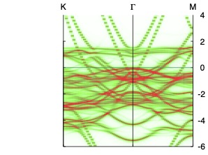
plbnds -range=-6,8 --h5 -fplot~scl=.5,.7~sh~ts=1 -ef=0 -scl=13.6 -dat=big -lt=1,col=0,0,0,colw=1,0,0,colw2=0,1,0,colw3=.9,.9,.9 -lbl bnds.h5

Either command generates fplot.ps, which you can view with your favorite reader. The small cell should look like the figure on the left; the zone-folded large cell should look like the figure on the right.

Note for the right figure, a third color weight of .9,.9,.9 was included, which corresponds to $w$. Including this weight (nearly) bleaches out bands that don’t belong to this k, i.e. $1-w_{n\mathbf{k}}$ close to unity. (Use colw3=1,1,1 to fully bleach them out.)

Green depicts s character, black p character and red d character. The bands on the right are essentially identical to those on the left, except for the (nearly) bleached out bands that belong to k₂…k₄.

Additional Exercises

1. Role of disorder

   To see the role disorder plays, add a small random magnetic field to each site. To do this, cut and paste the following to file bfield.co.

   % rows 8
   0  0 {1/2-ran(4)}/10
   0  0 {1/2-ran(0)}/10
   0  0 {1/2-ran(0)}/10
   0  0 {1/2-ran(0)}/10
   0  0 {1/2-ran(0)}/10
   0  0 {1/2-ran(0)}/10
   0  0 {1/2-ran(0)}/10
   0  0 {1/2-ran(0)}/10
   

   This supplies a random number on the third column (the z axis), which lmf will read as an external magnetic field. To see the actual numbers, try mcx bfield.co. The average absolute value of shift should be about 20 mRy, with the mean shift about 1 mRy.
   You also need to tell lmf to read this file. With your text editor, add the line below to the HAM category of ctrl.co.

    BFIELD= 2
   

   Before generating the bands, make a band pass to determine the Fermi level, as it will change because of the field.

   lmf -vfile=8 ctrl.co --quit=rho
   

Repeat steps 1 and 2 of the previous section. If you now inspect the weights, you will see that the weights outside the d band window (roughly −5 to +1 eV) continue to be close to 0 or 1, but the bands with lots of d character fluctuate between 0 and 1 a lot. This shows the d states are strongly scattered while the sp states are not. It is to be expected since the spin susceptibility in transition metals arises almost exclusively from the 3d states.

Draw the bands again. You should get something like the figure shown. Bands of sp character remain essentially unaffected, while bands of d character get blurred (except for some states around Γ that are energetically relatively isolated from other states).

2. The spectral function.

   A more compelling way to visualize the effects of disorder is by constructing the spectral function. As noted in the theory section, the extra bands from the supercell with partial weights present a form of disorder that can be cast as a Green’s function in the primitive cell, albeit with k and $\omega$-dependent self-energy, or hamiltonian. Thus the BZ unfolding technique is a another way, distinct from many-body perturbation theory, CPA or DMFT, to fold scattering from disorder into a self-energy Σ. In general Σ represents the difference between the one-body or non-interacting hamiltonian whose wave function factors into products of independent particle wave functions, and an “interacting” one in which the particles scatter via some potential not included in the one-body part. In GW and DMFT these originate from many-body effects which reflect the fact that the Schrodinger equation is not separable into a sum of one-body terms. The one-body hamiltonian of DFT or QSGW makes such a separation, but it is only approximate. In the present context, the hamiltonian is from one body (DFT) hamiltonian, and scattering originates a random B field.
   
   lmfgws, the postprocessing utility that analyzes dynamical self-energies, has a facility for reading bands constructed from BZ unfolding and generating a spectral function.

   lmfgws ctrl.co '--sfuned~units@eV~readebr@fn=bnds@useef@irrmesh~eps=0.02~se^band@fn=syml^nomg=5001^range=-6,4'
   

   The editor instruction  readebr@fn=bnds@useef@irrmesh  tells lmfgws to read eigenvalues and the last weight from bnds.h5. This input, and broadening  eps=0.02 eV (called $\delta$ in Eq. (9)), is used to make the Green’s function Eq. (9) from which it can make $A^{\mathbf{k}}(\omega)$ from Eq. (7), for k points in syml.co.  useef  tells the editor to read the Fermi level from bnds.h5.
   
   The last instruction  se^band@fn=syml^nomg=5001^isp=1^range=-6,4  generates $A^{\mathbf{k}}(\omega)$, over an energy window (−6,4) eV, on a frequency mesh of 5001 points.
   lmfgws writes $A^{\mathbf{k}}(\omega)$ to spq.co.

You can use plbnds utility in the “spectral function” mode (or use a utility of your own) to make a heat map of the spectral function, e.g.

   plbnds -sp~atop=10~window=-6,4 -lbl=KGM spq.co ; gnuplot gnu.plt

Use your favorite postscript to view the figure in spf.ps. It should look similar to the figure shown.