Running the DMFT loop

Introduction

As explained in the introduction to QSGW+DMFT, the fundamental step of DMFT is the self-consistent solution of the local Anderson impurity problem. This is connected to the electronic structure of the material (bath) through the hybridization function, the impurity level and the effective interactions $U$ and $J$. The sequence of operations leading to the self-consistent impurity self-energy is called DMFT loop.

The DMFT loop is composed by the following steps:

• The lattice Green’s function is projected onto the local correlated subsystem ($G_{\mathrm{loc}}(i\omega_n)$), where $\omega_n=(2n-1)\pi/\beta$ are the fermionic Matsubara’s frequencies. This leads to the definition of the hybridization function ($\Delta(i\omega_n)$) and the impurity levels ($E_{\mathrm{imp}}$).
• These two quantities together with the effective interactions $U$ and $J$ are passed to the Continuous Time Quantum Monte Carlo (CTQMC) solver which computes the corresponding impurity self-energy and the impurity Green’s function ($G_{\mathrm{imp}}(i\omega_n)$).
• The double-counting self-energy is subtracted from it and the result is embedded into an updated lattice Green’s function. After adjusting the chemical potential, the loop starts again from the starting point until the self-consistent relation $G_{\mathrm{imp}}(i\omega_n)=G_{\mathrm{loc}}(i\omega_n)$ is met.

From a software perspective, these operations are accomplished in a four-step procedure. Each step relies on a specific program (lmfdmft, atom_d.py, ctqmc and broad_sig.x). The operations performed by each code and the input/output handling needed to cycle the loop are indicated schematically in the figure below.

Running the loop

The DMFT loop is composed by alternated runs of lmfdmft and ctqmc, the output of each run being the input for the successive. To do that, do the following steps:

1. Prepare and launch the lmfdmft run

We are using the hybridization expansion CT-QMC solver. So before launching the solver we need to prepare the hybridization matrix for the Ni 3-d correlated orbitals. For that we need to launch the same lmfdmft command once more:

cd dmftrun
mpirun -n 24 lmfdmft -vnkabc=24 --rs=1,0 --ldadc=28.95 -job=1 ctrl.ni

This would take around 40 seconds to complete the job and produce the hybridization matrix (delta.ni) and chemical potentials (eimp1.ni) for the correlated impurity states. There are 5 d-orbitals and two spins, so the delta.ni file has 21 columns in total and is written in the same format as sig.inp. eimp1.ni file has information about the energies of the impurity levels.

Now we need to rename few files and edit some files to make sure the solver reads what it looks for. Also the PARAMS file that knows about all the parameters for CT-QMC and DMFT should read the energies for the impurity levels and chemical potential from the recently created eimpi.ni file:

cp delta.ni Delta.inp                                    
cp eimp1.ni Eimp.inp
echo "Ed [ -27.269069, -27.269069, -27.989260, -27.269069, -27.989262, -26.622308, -26.622310, -27.294755, -26.622312, -27.294760]" >> PARAMS                         # identify the impurity levels inside the PARAMS file
echo "mu   27.269069" >> PARAMS                           # identify the starting chemical potential inside the PARAMS file

At this point the PARAMS file should look like this

OffDiagonal  real
Sig  Sig.out
Gf  Gf.out
Delta  Delta.inp
cix  actqmc.cix
Nmax  300         # Maximum perturbation order allowed
nom  200          # Number of Matsubara frequency points sampled
exe  ctqmc        # Name of the executable
tsample  50       # How often to record measurements
M  1000000       # Total number of Monte Carlo steps per core
Ncout  100000            # How often to print out info
PChangeOrder  0.9         # Ratio between trial steps: add-remove-a-kink / move-a-kink
warmup  100000           # Warmup number of QMC steps
sderiv  0.02      # Maximum derivative mismatch accepted for tail concatenation
aom  10           # Number of frequency points used to determin the value of sigma at nom
U    4.0
J    0.3
nf0  8.0
beta 50.0
Ed [ -27.269069, -27.269069, -27.989260, -27.269069, -27.989262, -26.622308, -26.622310, -27.294755, -26.622312, -27.294760]
mu   27.269069

The PARAMS file is self explanatory. However we should be careful while choosing numbers for U, J, n and $\beta$ and make sure they are consistent with the choice of our double counting correction (ldadc) and the information inside the ctrl.ni file. Once the PARAMS file is ready we can now run a script called atom_d.py, which will generate all the essential information about the Hilbert space for the correlated impurity. But before that we also should have the file called Trans.dat in the path which knows about the size of the correlated block and the transformation matrix that connects the real harmonics to the spherical Harmonics for the correlated d-orbitals. For Nickel it looks similar to what is shown below, where the block containing numbers from 1 to 5 stands for one kind of spin and 6 to 10 for the other kind.

  10 10 #  size of Sigind and CF
#---- Sigind follows
  1    0    0    0    0    0    0    0    0    0
  0    2    0    0    0    0    0    0    0    0
  0    0    3    0    0    0    0    0    0    0
  0    0    0    4    0    0    0    0    0    0
  0    0    0    0    5    0    0    0    0    0
  0    0    0    0    0    6    0    0    0    0
  0    0    0    0    0    0    7    0    0    0
  0    0    0    0    0    0    0    8    0    0
  0    0    0    0    0    0    0    0    9    0
  0    0    0    0    0    0    0    0    0   10
#---- CF follows
  0.00000000  0.70710679   0.00000000  0.00000000   0.00000000  0.00000000   0.00000000  0.00000000   0.00000000 -0.70710679   0.00000000  0.00000000   0.00000000  0.00000000   0.00000000  0.00000000   0.00000000  0.00000000   0.00000000  0.00000000
  0.00000000  0.00000000   0.00000000  0.70710679   0.00000000  0.00000000   0.00000000  0.70710679   0.00000000  0.00000000   0.00000000  0.00000000   0.00000000  0.00000000   0.00000000  0.00000000   0.00000000  0.00000000   0.00000000  0.00000000
  0.00000000  0.00000000   0.00000000  0.00000000   1.00000000  0.00000000   0.00000000  0.00000000   0.00000000  0.00000000   0.00000000  0.00000000   0.00000000  0.00000000   0.00000000  0.00000000   0.00000000  0.00000000   0.00000000  0.00000000
  0.00000000  0.00000000   0.70710679  0.00000000   0.00000000  0.00000000  -0.70710679  0.00000000   0.00000000  0.00000000   0.00000000  0.00000000   0.00000000  0.00000000   0.00000000  0.00000000   0.00000000  0.00000000   0.00000000  0.00000000
  0.70710679  0.00000000   0.00000000  0.00000000   0.00000000  0.00000000   0.00000000  0.00000000   0.70710679  0.00000000   0.00000000  0.00000000   0.00000000  0.00000000   0.00000000  0.00000000   0.00000000  0.00000000   0.00000000  0.00000000
  0.00000000  0.00000000   0.00000000  0.00000000   0.00000000  0.00000000   0.00000000  0.00000000   0.00000000  0.00000000   0.00000000  0.70710679   0.00000000  0.00000000   0.00000000  0.00000000   0.00000000  0.00000000   0.00000000 -0.70710679
  0.00000000  0.00000000   0.00000000  0.00000000   0.00000000  0.00000000   0.00000000  0.00000000   0.00000000  0.00000000   0.00000000  0.00000000   0.00000000  0.70710679   0.00000000  0.00000000   0.00000000  0.70710679   0.00000000  0.00000000
  0.00000000  0.00000000   0.00000000  0.00000000   0.00000000  0.00000000   0.00000000  0.00000000   0.00000000  0.00000000   0.00000000  0.00000000   0.00000000  0.00000000   1.00000000  0.00000000   0.00000000  0.00000000   0.00000000  0.00000000
  0.00000000  0.00000000   0.00000000  0.00000000   0.00000000  0.00000000   0.00000000  0.00000000   0.00000000  0.00000000   0.00000000  0.00000000   0.70710679  0.00000000   0.00000000  0.00000000  -0.70710679  0.00000000   0.00000000  0.00000000
  0.00000000  0.00000000   0.00000000  0.00000000   0.00000000  0.00000000   0.00000000  0.00000000   0.00000000  0.00000000   0.70710679  0.00000000   0.00000000  0.00000000   0.00000000  0.00000000   0.00000000  0.00000000   0.70710679  0.00000000

• Run atom_d.py using the command

  atom_d.py J=0.8 l=2 OCA_G=False "CoulombF='Ising'" "Eimp=[   0.000000,   0.000000,  -0.720192,   0.000000,  -0.720194,   0.646761,   0.646759,  -0.025686,   0.646757,  -0.025691]"
  

  where the argument Eimp is a copy of the third line of Eimp.inp (to be changed at each iteration accordingly to the previous lmfdmft run) and the argument J is the Hund’s coupling. l=2 means the correlated impurity contains d-electrons. If the correlated impurity contains f-electrons (say for elemental Cerium) then l should be changed to 3. OCA_G=False implies that we don’t want to use One Crossing Approximation (OCA) as the impurity solver. CoulombF='Ising' implies that the interaction matrix is density-density. Alternatively, we can use CoulombF='Full' to work with a full slater-inetraction matrix for the correlated impurity.

  Running atom_d.py generates two files; actqmc.cix and info_atom_d.py used by the ctqmc solver. Now, let’s launch the CT-QMC solver.

  mpirun -n 24 ctqmc
  

• This job will run roughly for 7-8 minutes and produce the local Green’s functions (Gf.out) and self energies (Sig.out) among many other files. Important parameters (that may need to be adjusted during the loop) are nom, Nmax and M. Their explanation is reported as a comment in the PARAMS file itself but further information is available in the next tutorial. For this tutorial, you can set them to nom 200, Nmax 300 and M 1000000 (as illustrated in one dropdown box above).

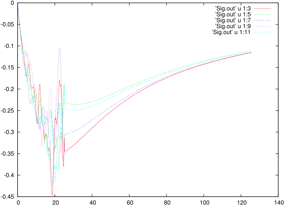
The imaginary part of the self energy would look ugly and something like this:

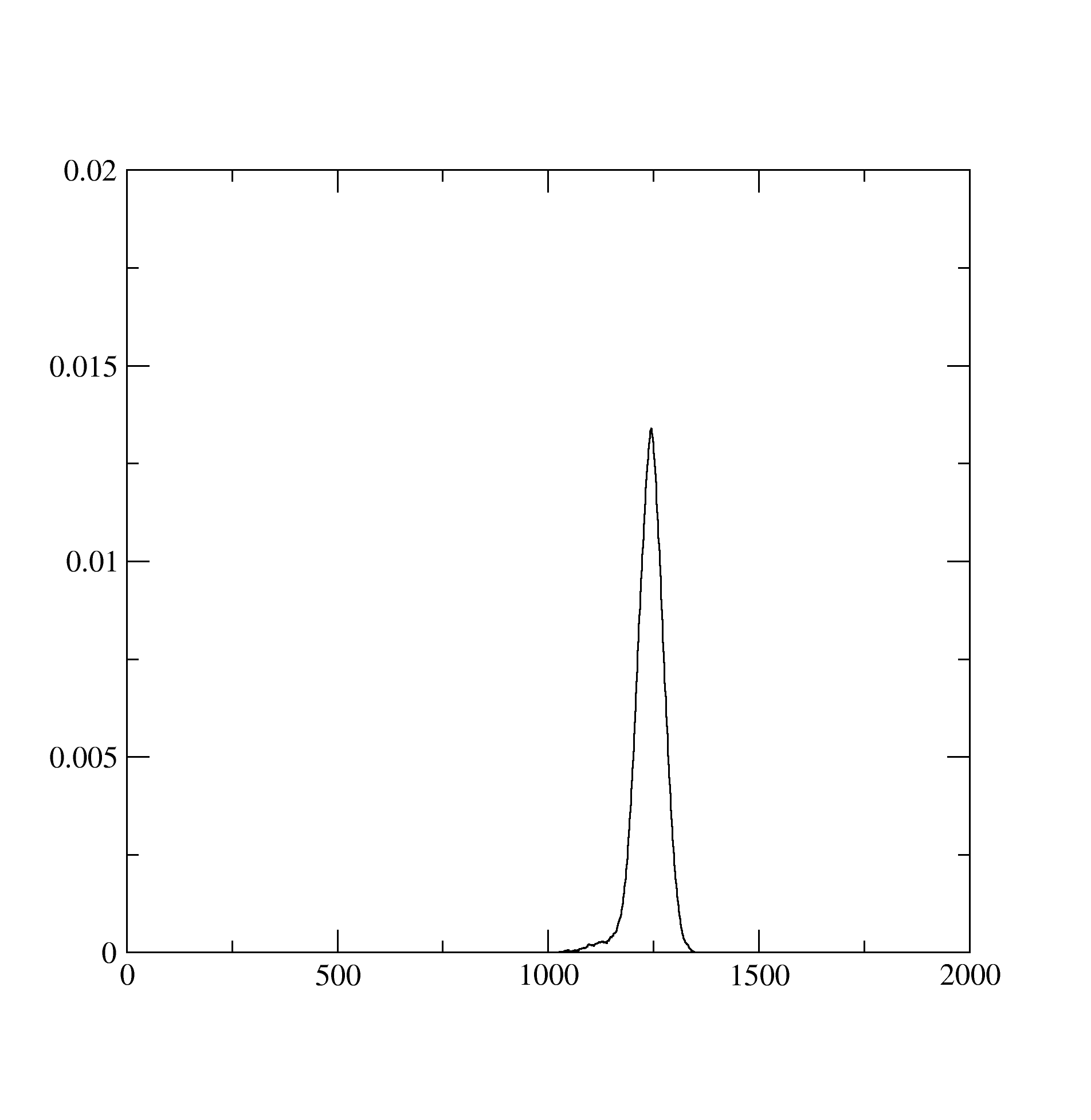
The histogram.dat stores information about the expnasion orders in hybridization that contributed dominantly to the solution. It looks like below and suggests that at least the expansion upto 1200 th order contributed:

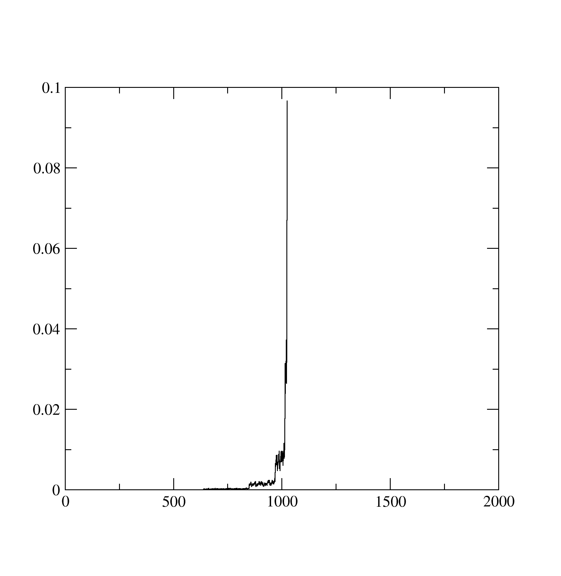
The Probability.dat stores the information about probabilities of occurence of different atomic states:

Among them we are especially interested in Sig.out, histogram.dat and the status files. To learn how to use them to judge on the quality of the QMC calculation we refer to the third tutorial. However, if we plot the data from Sig.out and Gf.out we can find that the data is extremely noisy. CT-QMC is, at the end of the day, a non-deterministic technique based on statistical sampling, and the primary way to improve the data quality is to increase the M 1000000 # Total number of Monte Carlo steps per core to a very large number. However, this primarily removes noise from the low energy part of the dynamic quantities but the noise at intermediate frequencies and the quality of the large energy tail, might need more care and alternative ways of betterment.

• Now there is a provision that we can broad Sig.out to smooth out the noise from intermediate frequencies. However, it is not at all must and one can always remove noise from intermediate frequencies by expanding dynamic local self energies or Green’s functions in the SVD basis. If you, however, use the program brad_sig.x you will run it with following commands

  echo 'Sig.out 150 l "55  20  150" k "1 2 3 2 3"'| broad_sig
  

  For a clearer explanation of how to use broad_sig.x, we refer to its commented header.

2. Cycling the loop

At this point you have a new self-energy to be fed to lmfdmft. All you want to do is to rename the newly produce Sig.out as sig.inp, and run lmfdmft with that as input. You will get a new set of hybridization (delta.ni) and chemical potentials (eimp1.ni). And you repeat the same process as discussed above to run another step of CTQMC+DMFT. This continues till you feel that the dynamic quantities are converged to your desired accuracy.

However, once you have familiarised with the procedure, you can write a script to do most of the work using this one as a basic template.

Converging to the SC-solution

The self-consistent condition holds when $G_{\mathrm{loc}}(i\omega_n)$ of iteration N is equal (within a certain tolerance) to $G_{\mathrm{imp}}(i\omega_n)$ of iteration N-1. You can add the flag --gprt when running lmfdmft to get $G_{\mathrm{loc}}(i\omega_n)$ printed on a file called gloc.ni. This can be compared with the file Gf.out produced by the previous CTQMC run. However in the comparison remember that the latter is not broadened, while the former is obtained by smoothened quantities.

An easier though accurate way is to look at the convergence of the chemical potential. This can be done by typing grep ' mu = ' it*_lmfrun/log.

A third method is of course to visualise the convergence of each separate channel of local quantities like Sig.out.brd or Gf.out.

In this tutorial, a reasonable convergence is achieved after around 10 iterations.