lmgf tutorial
This Introductory tutorial explains how to use the ASA Green’s function code lmgf. If you haven’t already done so, you are advised to go through the Introductory tutorial for the band code lm first.
- Create the input file. blm requires init.copt.
blm --mag --nk=8 --asa --gf copt
cp actrl.copt ctrl.copt
- Self-consistent density with lm.
lmstr ctrl.copt
lm ctrl.copt -vnit=0
lm ctrl.copt -vnit=30 --pr31,20
- Find the Fermi level with lmgf. Note the slight deviation from the tutorial so the code runs without user input.
sed -i 's/\(GFOPTS=.*\)/\1padtol=1d-5;/' ctrl.copt
rm -f mixm.copt log.copt
lmgf ctrl.copt -vnit=30 --pr31,20 --iactiv=no -vef=-.1293 --quit=rho
lmgf ctrl.copt -vnit=30 --pr31,20 --iactiv=no -vef=-.1293 --quit=rho
- Exchange interactions. Plot of spin wave spectrum requires syml.copt.
rm -f vshft.copt
lmgf -vgfmode=10 ctrl.copt -vef=-.1289
lmgf -vgfmode=11 ctrl.copt -vef=-.1289
echo 0 350 5 10 | plbnds -scl=13.6 -fplot~sh -lbl=X,G,M,R,G bnds.copt
Table of Contents
Summary
This package implements the ASA local spin-density approximation using Green’s functions. The Green’s functions are constructed by approximating KKR multiple-scattering theory with an analytic potential function. The approximation to KKR is essentially similar to the linear approximation employed in band methods such as LMTO and LAPW. It can be shown that this approximation is nearly equivalent to the LMTO hamiltonian without the “combined correction” term. With this package a new program, lmgf is added to the suite of executables. lmgf plays approximately the same role as the LMTO-ASA band program lm: a potential is generated from energy moments , , and of the density of states. in the same way as the lm code. You can use lmgf to make a self-consistent density as you can do with lm. lmgf is a Green’s function method: Green’s functions have less information than wave functions, so in one sense the things you can do with lmgf are more limited: you cannot make the bands directly, for example. However lmgf enables you do things you cannot do with lm. The most important are:
- Calculate magnetic exchange interactions
- Calculate magnetic susceptibility (spin-spin, spin-orbit, orbit-orbit parts)
- Calculate properties of disordered materials, either chemically disordered or spin disorder from finite temperature, within the Coherent Potential Approximation, or CPA.
- Calculate the ASA static susceptibility at to help converge calculations to self-consistency.
You can find some extra information on the way lmgf works in the lmgf documentation.
lmgf is a Green’s function program complementary to the ASA band code lm. For some properties, e.g. calculating moments lmgf can be straightforwardly substituted for lm because both calculate the DOS. The DOS is : it can be decomposed into site contributions and thus moments can be generated for each site and l channel, as an alternative to decomposing the eigenfunctions of the bands, as lm does. Thus it can achieve self-consistency in a manner similar to lm, but generating by an alternate route. If the ASA hamiltionian built by lm is suitably simplified, i.e. by
- omitting the “combined correction term” (OPTIONS_ASA_CCOR)
- generating from true power moments as the Green’s function does (HAM_QASA=0),
then lmgf and lm will produce nearly identical self-consistent solutions. When potential functions are parameterized to 2nd order in both lm and lmgf, and both methods are fully k converged, they should product nearly identical results. By default lm parameterizes the potential function to 3rd order; lmgf can do the same. The 3rd order parameterizations are similar in the two methods, but not identical. To verify this, try the following test:
gf/test/test.gf co 1 2 ← Test 1 for 2nd order parameterization; test 2 for 3rd order
lmgf is a bit messier to work with (Green’s functions are harder to stabilize than wave functions), and it a bit less accurate as the simplifications to lmf amount to approximations. Typically lm makes a better self-consistent potential.
But lmgf can do things lm doesn’t do, e.g. calculate magnetic exchange interactions through linear response as this tutorial demonstrates. Sometimes there is a need or advantage to carrying self-consistency via lmgf, e.g. when performing CPA calculations. Unless there is good reason to do otherwise, it is better use the self-consistent potential generated by lm to calculate other properties such as the magnetic exchange parameters. We follow that strategy here.
Preliminaries
For this tutorial the blm, lmchk, lmstr, lm and lmgf executables are required and are assumed to be in your PATH; the source code for all Questaal executables can be found here.
Tutorial
1. Building input file
Before starting working with this tutorial we advise you to read through the ASA-tutorial which explains building the input file in more details (you can also look through the input described in a full-potential context). In the present tutorial we’ll focus on the part of the input specific for using with lmgf.
To get started, copy the contents of the box below into file init.copt in your working directory. This file contains just the minimum structural information, apart from one line supplying some information about the magnetic structure:
LATTICE
        ALAT=7.1866
        PLAT=    1.000000   0.000000   0.000000
                 0.000000   1.000000   0.000000
                 0.000000   0.000000   1.000000
SPEC ATOM=Co MMOM=0,0,2.2
SITE
     ATOM=Pt POS=  0.0  0.0   0.0
     ATOM=Co POS=  0.5  0.5   0.0
     ATOM=Co POS=  0.0  0.5   0.5
     ATOM=Co POS=  0.5  0.0   0.5
Then use the blm utility (described in more detail in ASA-tutorial and full-potential tutorial. )
blm --mag --nk=8 --asa --gf copt
blm should generate file actrl.copt. Command-line switches blm recognizes are summarized in the Command line switches page.
The command-line switches are not required, but they supply quantities blm cannot determine automatically, that you will have to supply at some point. If you supply them on the command-line they are folded into the ctrl file at the outset; or, you can edit the ctrl file after it is generated.
- The --asa switch
This switch tailors the ctrl file for the ASA. To see how it affects the ctrl file, try running blm without --asa. For more details see the Introductory ASA tutorial.
- The --mag switch
- This switch tells blm that you plan on doing a spin polarized calculation. It mainly changes the preprocessor variable nsp to 2. This turns on the spin polarization through NSPIN={nsp}.
Without any other information the spin polarized calculation will proceed with zero magnetic moment. The system needs a “push” in the initial direction to find the magnetic state. You have to supply some initial information about the magnetic structure. Since we know that the magnetization is concentrated on the Co (Pt is paramagnetic, though it has a high magnetic susceptibility), the init file supplies an initial magnetic moment on the Co site of about 2 Bohr on the Co d orbital, in the SPEC category (SPEC ATOM=Co MMOM=0,0,2.2 in the initial file). The precise value 2.2 is not important: this quantity is determined self-consistently later. Choosing it rather large (the bulk moment is 1.8 ) gives it a strong initial push so to encourage it not revert to a (metastable) nonmagnetic state in the course of a self-consistent calculation.
- The --gf switch
- When --gf is used, blm prepares the input file for the Green’s function program lmgf. This tutorial uses lmgf to calculate magnetic exchange interactions. Adding --gf to the blm command line argument modifies actrl.copt in two ways:
1. The GF category is created:
  % const gfmode=1 nz=16 ef=0 c3=t   # lmgf-specific variables
  ...
  GF    MODE={gfmode} GFOPTS={?~c3~p3;~p2;}
To see the purpose of GF_MODE, do:
lmgf --input
and look for GF_MODE. You should see:
      GF_MODE           reqd   i4       1,  1          default = 0
             0: do nothing
             1: self-consistent cycle
             10: Transverse exchange interactions J(q), MST
             11: Read J(q) from disk and print derivative properties
             ...
So, if MODE=1, lmgf does a self-consistent calculation, generating the P and for each l channel using Green’s functions rather than wave functions as lm does.
GFOPTS bundles a variety of lmgf-specific options, which you supply through a sequence of strings separated by semicolons. The option it knows about are described in the input file documentation.
This tag:
GFOPTS={?~c3~p3;~p2;}
becomes GFOPTS=p3 after parsing by the preprocessor, because c3 is nonzero (see preprocessor documentation). p3 tells lmgf to use order potential functions (somewhat more accurate than order, but also prone to generating false poles not too far from the real axis).
2. EMESH is added to BZ:
  % const nz=16 ef=0
          EMESH={nz},10,-1,{ef},.5,.3  # nz-pts;contour mode;emin;emax;ecc;bunching
The energy contour
Green’s functions are energy resolved; thus physical properties such as the charge density or magnetic exchange interactions require an integration over the energy as well as over the BZ. For both density and static exchange interactions, the integration must be taken on the real axis from below the lowest eigenstate in the system to the Fermi level . Im G is basically the density-of-states. It is very spikey on the real axis, and a very fine energy mesh would be required to integrate Im G close to the real axis. The integration can be accomplished with vastly greater ease by deforming the contour into an elliptical path in the complex plane. A gaussian quadrature is used; typically 15 or so energy points is sufficient for a well converged result.
This contour is specified through EMESH. Breaking down the constituents of EMESH as autogenerated by blm:
     EMESH={nz}          ←  number of energy points in the contour; {nz} evaluates 16 in this file
            10           ←  elliptical contour
            -1           ←  starting energy on the contour.  Must be deeper than the lowest state in the system (-0.776 Ry)
           {ef}          ←  Fermi level determined by charge neutrality; see below
           0.5           ←  eccentricity of the ellipse ranging from 0 (circle) to 1 (line)
           0.3           ←  bunching parameter, bunching points near Ef. 0→no bunching
We don’t know what is a priori. In the ASA, a general reasonable guess is 0. If we perform the band calculation (see ASA-tutorial, we get generated by lm: it is about −0.13 Ry as we will soon see. is fixed by charge neutrality. If lmgf generated exactly the same spectrum as lm, and the k-integration were fully converged (or at least identical in the two cases) would be the same for lm as for lmgf. However we can expect that the charge neutrality points will slightly different in the two methods. Thus lmgf must be able to find its own Fermi level.
If you want to practice finding using lm use the following commands (for the details see ASA-tutorial). You can proceed directly to ASA self-consistency using lmgf, but we advise you to do those steps since you’ll need some of them further anyway but the following lm-part contains some useful information.
2. Self-consistent calculation using the ASA band program
Invoking blm with the switches given above is sufficient to make a working input file. So you can copy actrl.copt to ctrl.copt as it is.
All the ASA electronic structure codes (lm, lmgf, and lmpg) use a tight-binding form of the LMTO basis, where the envelope functions are screened to make them short ranged. This information is carried through screened structure constants, which in this package are precomputed and stored using lmstr. Run this setup to make the structure constants:
lmstr ctrl.copt ← Make and store structure constants
It should store str.copt and sdot.copt on disk. (If not, something is wrong and you should not proceed.)
As of yet we have no starting density or potential. You can see this immediately by trying to run the band code straight off:
lm ctrl.copt
The program will stop with this message:
LM: Q=ATOM encountered or missing input
In usual LDA calculations, a trial density is obtained by generating densities for free atoms, and superposing them (Mattheis construction). While the ASA code could have been written to do just this, it does something different. This code takes advantage of the simplification the ASA offers, namely that the sphere density is completely determined by a small number of parameters, namely the log derivative parameters P and energy moments of the charge density for each l channel. In the self-consistency cycle, only the are accumulated to construct the density for a new iteration). We can supply reasonable guesses through the ctrl file, or let the program pick some defaults as a first guess. Defaults are typically assigned so that is the charge in the l channel of the atom and are taken to be zero. While this is a pretty crude guess (cruder than the Mattheis construction) usually it is good enough that the program can find its way to the proper self-consistent solution.
The ASA code can either start from “potential parameters”, which gives it enough information to generate energy bands and calculate moments (, ) , or from the moments (, ) which is sufficient for the sphere routine to fix the potential and calculated potential parameters. The band and sphere blocks of the code are thus complementary: one takes the input of the other and generates output required by the other. The cycle is described on this web page.
The ctrl file is built with the following START category:
START CNTROL={nit==0} BEGMOM={nit==0}
If the argument to BEGMOM is zero, lm will start from potential parameters (which don’t exist yet, in the present case). Otherwise lm will start from the (, ). These haven’t been given either, but lm can pick defaults for them. We get an initial potential by doing:
lm ctrl.copt -vnit=0 ← Because -vnit=0, BEGMOM={nit} is preprocessed into BEGMOM=0
lm will start from (default) moments and generate a trial density for each sphere, together with potential parameters corresponding to potential generated.
The output should generate a table of potential parameters like this:
PPAR:  Pt        nl=4  nsp=2  ves=  0.00000000
  l     e_nu          C        +/-del     1/sqrt(p)      gam         alp
  ...
  1 -0.33739981  0.66438341  0.17542338   6.2239786  0.13462478  0.13462478
  2 -0.21536750 -0.17914256  0.02841817   1.1299420  0.01358564  0.01358564
  ...
  1 -0.33739981  0.66438341  0.17542338   6.2239786  0.13462478  0.13462478
  2 -0.21536750 -0.17914256  0.02841817   1.1299420  0.01358564  0.01358564
  ...
and a similar table for Co. Particularly important are C, the band center of gravity C, and del, which is the bandwidth parameter , as explained on this page. You can see that sits far above zero while is a little below. It tells you that the Pt d orbital is important for bonding while the Pt p orbital is pretty far above from the Fermi level and of much less importance. A disk file is created for each class. It contains the (, ), the potential parameters, and possibly other things. Take a look at files co.copt and pt.copt. You can see what defaults were chosen for (, ).
We are now ready for a self-consistent calculation. Doing:
lm ctrl.copt -vnit=30 --pr31,20 ← NIT={nit} is preprocessed into NIT=30. --pr31,20 sets verbosity fairly low
will perform up to 30 self-consistent cycles; see this page for the program flow.
lm will continue until the RMS change in (, ) falls below tolerance ITER_CONVC, or until 30 iterations is reached.
If it’s converged you’ll get the following phrase at the end of your output:
Jolly good show! You converged to ...
In this demo convergence should be reached in 21 iterations.
Interpreting the output:
The output can provide some very useful information. For example, the self-consistent Co moment is 1.8 ; Pt has a moment (induced by the neighboring Co) of 0.356 . You can see it in the line of the following form
ATOM=PT Z=78 Qc=68 R=2.928343 Qv=-0.009029 mom=0.356 a=0.025 nr=491
ATOM=Co ...
Scrolling up you can find the density-of-states at the Fermi level is D(Ef)=79.729 (units of Ry−1 per unit cell), or about 1.3 eV−1/atom. Had the calculation been done without spin polarization, D(Ef) would be ~187, more than twice larger. This is a very large number and suggests there is a likely instability. Indeed, the system can lower its energy by spontaneously magnetizing. Consider the Stoner criterion for spontaneous magnetization, I D(Ef) > 1. In 3d transition metals I is about 1 eV. Thus the Stoner criterion is easily satisfied and the system should spontaneously magnetize. In magnetizes so strongly that the Co moment (1.8 ) is larger than that for elemental Co (1.6 ).
The same line also provides you with the Fermi energy:
BZINTS: Fermi energy: -0.129264; ...
3. The Green’s function program lmgf
If you did not go through step 2, you must make set up an initial potential. Do
lmstr copt
lmgf ctrl.copt -vnit=0         ← Because -vnit=0, BEGMOM={nit} is preprocessed into BEGMOM=0
Finding The Fermi level
This page explains how lmgf determines the Fermi level. In this section we present a concrete example.
If GF_MODE=1, lmgf will generate the for whatever you give it. However there is only one physically meaningful : the one that satisfies charge neutrality. The input file is constructed so you can supply through command-line argument -vef=_expr__{:.path}: the preprocessor evaluates ef from expr, substitutes it for {ef} in the input file (see preprocessor documentation). We’re going to use the one obtained by running _lm (see the previous section).
The simplest way to find the charge neutrality point is to run lmgf interactively in the self-consistent mode (GF_MODE=1). By running lmgf interactively you can monitor convergence. The band code from the previous section tells us that the Fermi level should be close to −0.1293. Do:
lmgf ctrl.copt -vnit=30 --pr31,20 --iactiv -vef=-.1293 --quit=rho
Since we’re using --iactiv switch the code is going to stop and ask us to make some choices. At first you’ll see
QUERY: max it (def=30)?
Just hit Enter (return) to confirm. Output contains two tables the first of which looks like
 GFASA:  integrated quantities to efermi = -0.1293
     PL      D(Ef)      N(Ef)       E_band      2nd mom      Q-Z
 spin 1   11.462633   21.527363   -7.139450    2.654618    3.027363
 spin 2   79.623007   15.413297   -4.696371    1.699848   -3.086703
  total   91.085640   36.940660  -11.835821    4.354465   -0.059340
 N(up)-N(dn)           6.114066
         deviation from charge neutrality: -0.05934
The non-zero deviation from charge neutrality means that ef=-.1293 results in a slight electron deficiency. lmgf will estimate a constant shift to crystal potential to make the system neutral, and interpolate G to contour adjusted by this shift using a Pade approximant.
It prints out the modified results after an estimate of the Fermi level is found interpolating to other energies using a Pade approximant
 Corrections to integrated quantities estimated by Pade interpolation
     PL      D(Ef)      N(Ef)       E_band      2nd mom      Q-Z
 spin 1    8.855135   21.530086   -7.151379    2.654673    3.030086
 spin 2  110.788350   15.469914   -4.712007    1.700791   -3.030086
  total  119.643484   37.000000  -11.863385    4.355464   -0.000000
 N(up)-N(dn)           6.060171
         deviation from charge neutrality: 0
At the prompt you should see
QUERY: redo gf pass (def=F)?
It is asking you whether you want to accept the Pade approximant, or redo the GF calculation with the potential shift added. Let’s do the latter, to see how good the estimate was. At the prompt type ‘st’ and hit return twice
QUERY: redo gf pass (def=F)? st <RET> <RET>
After the cycle you should see
deviation from charge neutrality: 0.015781
The Pade correction reduces the deviation from neutrality but overestimates the shift. A new estimate is made for the potential shift and the prompt reappears.
Note: lmgf shifts the average crystal potential, keeping is kept fixed.
At the third iteration you should see something like
gfasa: potential shift this iter = 0.000004. Cumulative shift = -0.000422
`Cumulative shift’ is the net shift accumulated over all the iterations. You can repeat the GF cycle as many times as you like. (If you see QUERY: modify vbar (def=…)? just hit return) If you iterate a few times you should see the deviation get small. The contribution from the third iteration is already negligible and we stop here.
Note: If you skipped the initial self-consistency with lm, these numbers will all be different. But the idea remains the same.
When you are satisfied with the smallness of the deviation enter either
QUERY: redo gf pass (def=F)?   q <RET>
which stops execution immediately, or
QUERY: redo gf pass (def=F)?   <RET>
to continue towards self-consistency.
Consider the first case. The constant potential shift is just the negative the requisite Fermi level shift to achieve charge neutrality. needs to be adjusted to −0.1293−(−0.0004) = −0.1289 Ry.
To confirm that this is the correct Fermi level, repeat the interactive lmgf instruction with -vef=-0.1289. You should find that the deviation from charge neutrality is about −0.003 electrons, which is small.
Consider the second case. lmgf should print out something like the following and wait for another prompt
 gfasa:  potential shift this iter = 0.  Cumulative shift = -0.000434
 ...
 gfasa (exit): vconst updated from 0.000000 to -0.000434
 ...
 QUERY: redo, nmix= (def=2)?
Quit execution by entering q <RET> at the prompt.
lmgf stores the potential shift as vconst in file vshft.copt. It remembers the potential shift for the given Fermi level. Now run lmgf exactly as you did the first time (do not change ef) and you should see that the deviation from charge neutrality is small.
You can now proceed to self-consistency but we will instead use the potential generated by lm in order to make the exchange parameters.
If you do proceed to self-consistency using lmgf, vshft.copt keeps track of the potential shift through each iteration. After self-consistency is reached you can either keep vshft.copt, or remove it and modify the Fermi level so charge neutrality is satisfied without the shift.
4. Magnetic Exchange Interactions
As we mentioned before lmgf requires a GF-specific category (look into ctrl.copt).
GF MODE=1 GFOPTS=options
Token MODE= controls what lmgf calculates. Options are MODE=1, MODE=10, MODE=11, MODE=26.
Look into ctrl.copt. Two lines are important here:
% const gfmode=1 c3=t
GF      MODE={gfmode} GFOPTS={?~c3~p3;~p2;}
MODE={gfmode} means that you can define MODE in the command line by adding -vgfmode=1|10|11|26. If you don’t include this switch lmgf will operate in mode 1 (from % const gfmode=1), as it in the previous section. Now we’ll need MODE=10 that invokes a special branch computing magnetic exchange interactions using a linear response technique.
The Heisenberg model is an empirical model that postulates a set of interacting rigid local spins. The Hamiltonian is
The are called “Heisenberg exchange parameters”. The Heisenberg applies to a system of rigid spins undergoing small excursions about equilibrium. R and R’ are any pair sites and is a kind of magnetic analog to the dynamical matrix describing small oscillations of nuclei around their equilibrium point. In a crystal with periodic boundary conditions can be Bloch transformed to read:
, where R and R’ are now confined to sites within a unit cell.
lmgf calculates from the “Lichtenstein formula.” This famous expression (J. Magn. Magn. Mater. 67, 65 (1987)), closely related the static transverse magnetic susceptibility , is derived from density functional perturbation theory. It establishes a first-principles basis for the Heisenberg model. One elegant (though approximate) feature of the ASA is that the magnetization is everywhere associated with an atomic sphere. For local moment systems, the magnetization is well confined inside a sphere; thus associated with every site R there is a well defined local moment. If sufficiently localized it rotates rigidly under the influence of an external perturbation.
When you set GF_MODE=10, lmgf will generate , and then perform an inverse Bloch transform (by Fast Fourier Transform) to make for as many lattice translation vectors T as there are k-points.
Do
rm -f vshft.copt
lmgf -vgfmode=10 ctrl.copt -vef=-.1289
Results are saved in file jr.copt (see below).
Most of the analysis is done in the next step, but already the output from gfmode=10 contains some useful information. In the first of this pair of tables you see J_0 and 2/3 J_0. J_0 is the net Weiss magnetic field from the surrounding neighbors; 2/3 J_0 would be the (classical) mean-field estimate for the critical temperature if there were one atom/cell. Since the Pt moment is very small it is weakly magnetic and has little effect on . In the second table (J_0 resolved by L) J_0 is decomposed into l and m contributions. As expected, the contributions to J_0 originate almost entirely from the d states.
Now if you run lmgf with GF_MODE=11, it reads jr.copt (which means you have to run MODE=10 first) and does some analysis with the parameters. Invoke lmgf with
lmgf -vgfmode=11 ctrl.copt -vef=-.1289
A unit cell of N sites has pairs. Thus jr.copt holds a succession of tables of J, one array for each RR’ pair in the unit cell. Each array has exchange parameters, corresponding to the lattice translation vectors that follow from the Fast Fourier Transform of a k mesh of points. You can find the headers for each array (headers follow a standard format this package uses) by doing, e.g.
grep rows jr.copt
to see:
% rows 64 cols 8 real  rs  ib=1  jb=1
% rows 64 cols 8 real  rs  ib=1  jb=2
 ...
Each array has 64×8 entries, for T vectors derived from 8×8×8 k-points (the 3D array is stored in a 2D format). lmgf unpacks these (GF_MODE=11) and prints them out in a sequence of tables, e.g. this one coupling all pairs of atoms belong to sites 2 and 3 in the unit cell. Pairs are ordered by separation distance d. Interactions fall off rapidly with d, and oscillate around 0, as might be expected from RKKY theory. Then follow estimates for the critical temperature . is estimated in Weiss mean-field theory, and also according to a spin-waves theory by Tyablikov (sometimes called the “RPA”). Mean-field tends to overestimate ; RPA tends to be a little more accurate but tends to underestimate it. From these two estimates should be around 1000K (see the GF_MODE=11 output).
Next follows an estimate for the spin wave stiffness. We need a symmetry lines file for the simple cubic structure. You can copy it from /lm/misc/ (assuming ~/lm is your build directory). The folder has symmetry files for different structures.
Copy the box below to syml.copt.
41  0.5 0 0    0 0 0                  X to Gamma
41   0 0 0    .5 .5 0                 Gamma to M
41  .5 .5 0   .5 .5 .5                M to R
41  .5 .5 .5   0 0 0                  R to Gamma
0 0 0 0 0 0 0
lmgf reads this file and calculates the spin wave spectrum from the Heisenberg model, along the lines specified. Results are saved in bnds.copt (the energy scale is now mRy). So let’s run GFMODE=11 again to get it (now we have the symmetry lines file):
lmgf -vgfmode=11 ctrl.copt -vef=-.1289
You can plot magnon spectra using the same technology you use for plotting energy bands, see ASA-tutorial. If you have the plbnds and fplot packages installed do:
echo 0 350 5 10 | plbnds -scl=13.6 -fplot~sh -lbl=X,G,M,R,G bnds.copt
Now you have fplot.ps file with the spectra (you can rename this file to some-name.ps) and use your favorite postscript reader to view it. You should see something close to what is shown in the figure:
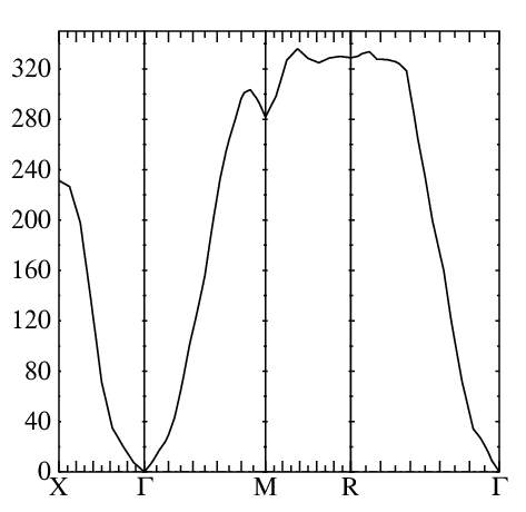 .
.
Magnon energies are in meV.
Note: The 8×8×8 mesh is a bit coarse. Use a finer k mesh for a smoother and more accurate magnon spectrum.