In this tutorial, we will apply dynamical mean field theory (DMFT) on Sr2RuO4 on a QSGW stating point that you can find here

or on Scarf

cp /work3/training/questaal/data/dmft_sr2ruo4.tar.bz2 .

Impurity solver

Questaal package does not supply an impurity solver. There are several choices of solvers on the market, in this tutorial, the CTQMC solver from the TRIQS package is used (see TRIQS package and its hybridization-expansion solver solver) TRIQS is already installed on the machine used for this workshop.

Prepare Input folder and files

Open dmft_sr2ruo4.tar.bz2

tar xvf dmft_sr2ruo4.tar.bz2
cd dmft_sr2ruo4

If you list your directory now, you should have :

atm.sr2ruo4  basp.sr2ruo4  ctrl.sr2ruo4  rst.sr2ruo4  sigm.sr2ruo4  site.sr2ruo4

Definition of the correlated subspace

At the end of ctrl file add the following lines:

DMFT    BETA=30 NOMEGA=999 NLOHI=16,42
        BLOCK:
        SITES=3 L= 2
        SIDXD= 1 2 0 2 0

Remark: Make sure you have the right indentation between the token DMFT and BLOCK.

Projection window

The first tokens are:

BETA=30 : The DMFT loop is done at inverse temperature (ev^-1) 30.
NOMEGA : Number of Matsubara frequencies for the impurity self energy.
NLOHI=16.42 : The projector are constructed with the bands from 16 to 42.
How to select NLOHI
In principle, the window is infinite and all the bands should be included. In practice, for numerical reasons, we choose a large finite windows around the d-state.
plot the partial dos on Ru atom (see tutorial here
mpirun -np 12 lmf sr2ruo4 -vnkabc=8 --quit=rho --pdos~mode=2~sites=3~lcut=2
lmdos sr2ruo4 -vnkabc=8 --quit=rho --pdos~mode=2~sites=3~lcut=2 --dos:npts=1001:window=-1,1
echo 1.4 5 -20 20 | pldos -fplot~sh~long~open~tmy=.25~dmin=0.40~xl=E -esclxy=13.6 -ef=0 -lst="5;6;7;8;9" dos.sr2ruo4
which prints a file fplot.ps that you can open with evince :
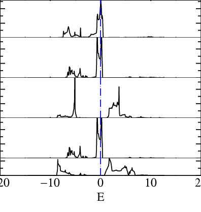
Panel 1,2,4 are t2g bands and 3,5 are eg.
In this tutorial, we will include the t2g bands so we want at least a windows at least of around -8 ev to 8 eV the following command :
mpirun -np 12 lmf ctrl.sr2ruo4 --minmax~ef0~ev --quit=rho
prints an array with the lower and higher energies of each bands over the Brillouin zone (in eV, relative to the Fermi level).
1 -44.3639-44.3497 | 65 24.6447 26.9751 | 129 63.4499 67.0030
2 -44.3621-44.3487 | 66 25.5025 27.5054 | 130 64.9246 68.3639
3 -43.9959-43.9922 | 67 25.9274 28.0126 | 131 65.8215 68.4935
4 -36.6674-36.5877 | 68 26.3476 28.4759 | 132 66.3480 69.2668
5 -36.6052-36.5623 | 69 27.0485 29.2219 | 133 67.0030 69.7670
6 -21.6012-20.4596 | 70 27.5175 30.5218 | 134 67.7296 71.1499
7 -20.5487-20.4463 | 71 27.9963 30.8646 | 135 68.1644 71.4900
8 -20.1141-19.6980 | 72 28.6419 31.2388 | 136 68.8294 72.4355
9 -19.9636-19.4625 | 73 28.6928 32.0471 | 137 68.9175 72.8961
10 -18.6634-18.1766 | 74 29.8014 32.4042 | 138 69.3634 73.0867
11 -18.5672-18.1023 | 75 30.2767 33.1881 | 139 69.6761 73.5590
12 -18.3387-18.0421 | 76 30.7850 34.2614 | 140 70.4414 74.0920
13 -18.2624-17.8759 | 77 31.2068 34.7062 | 141 71.9113 74.3569
14 -18.0055-17.3478 | 78 32.5198 35.1082 | 142 72.0429 75.0024
15 -17.7978-17.3328 | 79 33.1905 35.5611 | 143 73.3876 75.5247
16 -8.7415 -5.7184 | 80 34.2706 36.0721 | 144 73.7077 76.0873
17 -8.4662 -5.7184 | 81 34.5046 36.5411 | 145 74.6232 76.8166
18 -7.4729 -5.1152 | 82 34.6476 36.6204 | 146 75.4742 78.0036
19 -6.3248 -4.9609 | 83 35.0262 36.8990 | 147 76.2399 78.3877
20 -6.0095 -4.2071 | 84 35.3958 38.1754 | 148 76.5344 78.7125
21 -5.1659 -4.0326 | 85 35.4764 38.2633 | 149 76.9394 79.6267
22 -4.6066 -3.3940 | 86 35.6191 38.9050 | 150 77.7823 80.0811
23 -4.4619 -3.3072 | 87 35.9060 39.1817 | 151 78.4270 81.0298
24 -3.9376 -3.1200 | 88 36.5507 39.6747 | 152 78.6801 81.1216
25 -3.8228 -2.7379 | 89 37.3101 39.9634 | 153 78.8622 81.9173
26 -3.1909 -2.6617 | 90 37.3728 40.4092 | 154 79.5259 82.6096
27 -2.9680 -2.4403 | 91 37.9164 41.0772 | 155 80.1328 83.2408
28 -2.8285 0.3722 | 92 38.4716 41.4645 | 156 81.1495 83.6986
29 -0.8810 0.3963 | 93 38.9698 42.0651 | 157 81.9281 84.6429
30 -0.8806 0.5328 | 94 39.9048 42.5988 | 158 82.4948 85.1756
31 0.7721 3.7782 | 95 40.5127 43.0717 | 159 83.1580 87.0767
32 2.0161 5.7185 | 96 41.3112 43.7090 | 160 83.7712 87.5075
33 3.5324 6.1219 | 97 42.0524 44.4195 | 161 84.4264 88.0207
34 3.9819 6.9169 | 98 42.6085 46.2012 | 162 84.5085 88.9146
35 5.5211 7.7916 | 99 42.8757 47.3416 | 163 85.3575 89.8406
36 6.1828 8.3554 | 100 43.4706 47.3438 | 164 86.3552 90.2052
37 6.8933 8.9681 | 101 43.9656 47.8023 | 165 87.1299 90.5521
38 7.5018 9.2767 | 102 44.9182 49.1144 | 166 88.2587 91.8020
39 7.7328 10.0707 | 103 45.4036 49.3399 | 167 89.0026 92.5003
40 8.1388 10.5204 | 104 45.5959 50.2699 | 168 89.5906 93.3148
41 9.0049 10.8916 | 105 46.1506 51.3297 | 169 90.0144 94.4348
42 9.5772 11.1922 | 106 46.9452 51.6208 | 170 91.0070 94.7336
43 9.7116 11.6210 | 107 47.7742 51.8409 | 171 92.1758 95.8743
For this tutorial NLOHI=16,42

Definition of the impurity

In our example, the correlated subspace is composed of Ru t2g-states. This information is given by:

        BLOCK:
        SITES=3 L= 2
        SIDXD= 1 2 0 2 0

The DMFT subspace can have several correlated atoms. each correlated atoms is defined with it index in the site file, the orbital caracters of the corraleted orbital (l=2 for d, l=3 for f).

SITES : index of correlated site (Here Ru which is the atom 3 in site file
L : orbital momentum of correlated subspace (L=2 for d)
SIDXD indicates which m =[-l .. +l] are taken into account in the impurity self energy. 0 means that the orbital is not selected. index higher than 1 means the orbital is selected. Putting the same index to several orbital means that they are concidered to be equivalent. Since L=2, we can select the d orbital of Ru (xy,yz,z2,xz,x2-y2). We want to select only t2g orbital (xy,yz,xz) and here yz,xz are equivelent.
To included off-diagonal term, SIDXD has to be replaced SIDXM and a (2L+1)x(2L+1) matrix has to be supplied. Here we take into accout xy, yz, xz where yz and xz are equivalent. The order in given by Questaal’s ordering

Ctrl file for DMFT

# Autogenerated from init.sr2ruo4 using:
# /users/ms4/bin/blm --gw --express=1 --nk=12 --nkgw=6 --gmax=11.0 --nit=100 sr2ruo4
% const nit=100
% const met=5
% const so=0 nsp=so?2:1
% const lxcf=2 lxcf1=0 lxcf2=0
% const pwmode=0 pwemax=3
% const sig=12 gwemax=2.46 gcutb=3.1 gcutx=2.5
% const nkabc=12 nkgw=6 gmax=11 beta=.3
VERS  LM:7 FP:7 # ASA:7
IO    SHOW=f HELP=f IACTIV=f VERBOS=35,35  OUTPUT=*
EXPRESS
  file=   site
  nit=    {nit}
  mix=    B2,b={beta},k=7
  conv=   1e-5
  convc=  3e-5
  nkabc=  {nkabc}
  metal=  {met}
  nspin=  {nsp}
  so=     {so}
  xcfun=  {lxcf},{lxcf1},{lxcf2}
#SYMGRP i r4z mx
HAM   GMAX={gmax}
      AUTOBAS[PNU=1 LOC=1 MTO=4 LMTO=5 GW=1 PFLOAT=2,1]
      PWMODE={pwmode} PWEMIN=0 PWEMAX={pwemax} OVEPS=0
      XCFUN={lxcf},{lxcf1},{lxcf2}
      FORCES={so==0} ELIND=-0.7 NSPIN={nsp} SO={so}
      RDSIG={sig} SIGP[EMAX={gwemax}]
ITER  MIX=B2,b={beta},k=7  NIT={nit}  CONVC=1e-5
BZ    METAL={met}  NKABC={nkabc}
GW    NKABC={nkgw} GCUTB={gcutb} GCUTX={gcutx} DELRE=.01 .1
      GSMEAR=0.003 PBTOL=3e-4,3e-4,1e-3
STRUC
      SHEAR=1 0 0 1.0
      NL=5  NBAS=7  NSPEC=3
      ALAT= 7.30111097
      PLAT= -0.5  0.5  1.6455593  0.5  -0.5  1.6455593  0.5  0.5  -1.6455593
SPEC
  ATOM=Sr       Z= 38  R= 2.985910  LMX=3 LMXA=4
  ATOM=Ru       Z= 44  R= 2.068587  LMX=3 LMXA=4 PZ=0,0,5.4
  ATOM=O        Z=  8  R= 1.581969  LMX=3 LMXA=4
SITE
  ATOM=Sr         POS=  0.5000000   0.5000000  -0.4851109
  ATOM=Sr         POS= -0.5000000  -0.5000000   0.4851109
  ATOM=Ru         POS=  0.0000000   0.0000000   0.0000000
  ATOM=O          POS=  0.0000000   0.5000000   0.0000000
  ATOM=O          POS=  0.0000000   0.0000000   0.5348068
  ATOM=O          POS= -0.5000000   0.0000000   0.0000000
  ATOM=O          POS=  0.0000000   0.0000000  -0.5348068
DMFT    NLOHI=16,42 BETA=30 NOMEGA=999
        BLOCK:
        SITES=3 L= 2
        SIDXD= 1 2 0 2 0

Double Counting

We will use a static double counting given by the fully localized limit (FLL), with U = 4.5 eV, J = 1 eV, n = 4

Edc = U(n-1/2)-J(n-1)/2 = 14.25 eV

echo "14.25 14.25" > dc.sr2ruo4  # there is one value for each independent active orbital

Solver parameters

The CTQMC solver is a Monte Carlo solver. The parameters needed by the solver are given in para_triqs.txt. In this tutorial, we just need one params file. An example is given below :

U 4.5
J 1
n_warmup_cycles 100000
n_cycles 1000000
length_cycle 30
n_l 50

U : Effective interation
J : Hund coupling
n_warmup_cycles : number of warmup steps at the beginning of the Markov chain to reach an ergodic Markov chain.
n_cycles : total number of measures
length_cycle : number of steps between two measures. If this number is too small, the data will be noisy due to correlated sampling. If this number is too large, the calculation will be longer uselessly.
n_l : number of Legendre coefficients (see [3])

Put the parameters above in a file called para_triqs.txt

Note: The total number of measures is n_cycles. The Monte carlo process is highly parallelazible, adding more cores will decrease the number of measure per core.

First iteration

In general, it is adviced to perform the first iteration and check the quality of the result in order to be sure that the number set in para_triqs.txt are ok.

Create a new folder for the first iteration

mkdir it1
cp -f * it1/.
cd it1/

In it1, run lmfdmft to create a self energy file sig.inp

lmfdmft sr2ruo4 --ldadc~fn=dc --job=1

this command creates a file sig.inp

Structure of sig.inp

sig.inp is a text file which contains the self energy.

there is NOMEGA lines Then the structure of the collun is

w Re(S_1) Im(S_1) ... Re(S_i) Im(S_i)

where i is the index given in the token SIDXD or SIDXM

Once the file sig.inp is created, run again

mpirun -np 12 lmfdmft sr2ruo4 --ldadc~fn=dc --job=1

It will create the file solver_input.h5 which is a hdf5 file format.

G_{loc} = \sum_k \frac{1}{i\omega - \epsilon_k -\Sigma_{DMFT}(i\omega)}

\mathcal{G}_0 = ((G_{loc})^{-1} + \Sigma_{DMFT}(i\omega)) ^{-1}

Structure of solver_input.h5

not fixed yet.

Let try to run the ctqmc solver now.

mpirun -np 12 lmtriqs sr2ruo4

The calculation takes about 10 minutes. In the plot show below, we run the calculation on 12 cores.

The first thing to check is that the number of Legendre coefficient for the Green function is correct. it has to be high enough so the coefficient goes to zeros. If it is too high, the highest coefficients contain just Monte Carlo noise which pollutes the final result.

Plot of G_l

The file gl.inp contains g_l with the following format :

nb_of_legendre_coef Re(G_l_1_up) ... Re(G_l_i_up) .... Re(G_l_1_down) ...

A python script to plot it could be :

import numpy as np
import matplotlib.pyplot as plt
import sys
Gl = np.loadtxt(sys.argv[1]).T
wl = Gl[0]
Gl = Gl[1:]
#plot just G_l_up
for i in range(Gl.shape[0]) :
    plt.plot(wl,Gl[i])
plt.xlabel('n_l')
plt.ylabel('Gl')
plt.savefig('gl.png')
plt.show()

put this script in a file plot_gl.py and run

python plot_gl.py path_to/gl.inp

You should obtain :

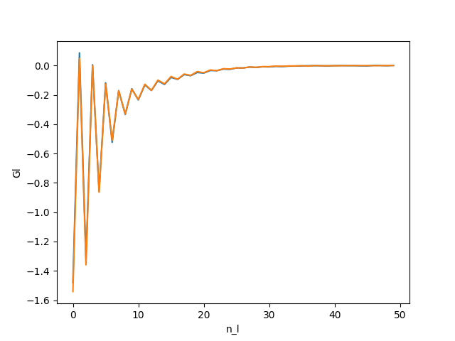G_l All the coefficients go to 0.

Then, the Green function on the Matsubara axis is deduced from G_l and the self energy is obtained from the Dyson equation.

The self energy is contained in the file sig.inp

Plot sig.inp

A simple python script to plot sig.inp could be :

import numpy as np
import matplotlib.pyplot as plt
import sys
S = np.loadtxt(sys.argv[1]).T
w = S[0]
Sig = S[1::2] + 1j* S[2::2]
#plot just Sig_up
plt.figure(figsize=(8,8))
for i in range(Sig.shape[0]) :
    plt.plot(w,Sig[i].imag,label=i+1)
plt.xlabel(r'$\Omega_n$', fontsize = 20)
plt.ylabel(r'$\Sigma$', fontsize = 20)
plt.xlim(0,200)
plt.legend()
plt.savefig('sig_sr2ruo4.png')
plt.show()

put this script in a file plot_giw.py and run

python plot_giw.py path_to/sig.inp

You should obtain :

Self energy

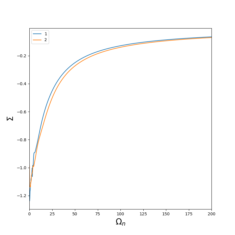
The self energy of the second orbital is noiser than the first one because the second one is the average of yz and xz.

To complete the dmft loop, we need to run again lmfdmft to get a updated hybridisation function and energies of the impurities and then run again the impurity solver to get a new self energy. It has to be repeated until convergence.

DMFT loop

To perform the DMFT loop, we proposed a bash script which could be adapted for your machine. It’s assumed that you have set correctly the ctrl file and the params file

#!/bin/bash -l
set -xe
x=sr2ruo4
mxit=20 # nb of iteration
np_lmfdmft=12 # nb of cores available for lmfdmft
np_ctqmc=12 # nb of cores available for lmfdmft
if [ ! -e it1 ]; then
    mkdir -p it1
    cp -f * it1/.
fi
for i in `seq $mxit`;
do
    [ ! -e "it$((i-1))" ] || [ ! -e "it${i}"  ] || continue # if some iterations have already be done ...
    [ ! -e "it$((i-1))" ] || [ -e "it${i}"  ] || cp -av "it$((i-1))" "it${i}"
    pushd "it${i}"
    mpirun -n $np_ctqmc  lmfdmft --ldadc~fn=dc -job=1 ctrl.$x
    rm -f evec* proj*
    mpirun -np $np_ctqmc lmtriqs $x
    popd
done

It is adviced to check the convergence by plotting the difference sig.inp in each itX folder. It is also adviced to perform the average over the last iteration.

You can find a converged result in

extra/sig_converge.inp

For the rest of the tutorial, replace your sig.inp by the converge one:

cp extra/sig_converge.inp sig.inp

This has been converged using 30 iterations and average on the 10 last interation (with n_cycles=50000000) on a 12 cores machine.

Analyse of the result

Analytic continuation

In this tutorial we use lmfdmft’s built in Pade extrapolator to carry out the analytic continuation.
Note: analytic continuation is a tricky business. Pade works reliably only when the polynomial order is not too large, which means in can operate reliably only over a small energy window. Also the self-energy should be reasonably smooth.

lmfdmft sr2ruo4  --rs=1,0 --ldadc~fn=dc -job=1 --pade~nw=121~window=-6/13.606,6/13.606~icut=30,75

it creates a file sig2.sr2ruo4 containing the self energy in the real axis which has the same format than sig.inp.

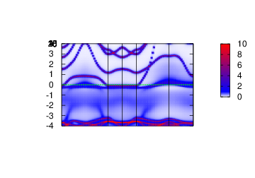
Spectral function

In this section, the spectral function $A(w,k) = - \frac{1}{\pi} \frac{1}{\omega - \epsilon_k -\Sigma_{DMFT}(\omega)}$

To do so, execute the following command.

 cp extra/syml.sr2ruo4 . # copy the symetry lines.
 mpirun -np 12 lmfdmft sr2ruo4  --rs=1,0 --ldadc~fn=dc -job=1 --gprt~band,fn=syml~rdsigr=sig2~mode=19
 lmfgws sr2ruo4 '--sfuned~units eV~readsek@useef@irrmesh@minmax~eps 0.02~se band@fn=syml nw=2 isp=1 range=-4,4'
 plbnds -sp~atop=10~window=-4,4 spq.sr2ruo4
 gnuplot gnu.plt

Spectral function

Density of States

To obtain the density of states, you can run lmfdmft with the flags –gprt~rdsigr=sig2~mode=18

lmfdmft sr2ruo4 -vnkabc=8 --ldadc~fn=dc --job=1 --gprt~rdsigr=sig2~mode=18

Note: you can speed up the calculation by using mpi for lmfdmft

It will dump the DOS in the file dos.h5 which can be read using a simple python script

A python script to plot it could be :

import numpy as np
import h5py
import matplotlib.pyplot as plt
def r(f) :
    f=h5py.File(f)
    d = np.sum(np.array(f['dos']),axis=(0,1))
    w = np.array(f['omega'])
    d = d.real/np.sum(d[1:]*(w[1:]-w[:-1])) # normalized DOS to 1
    return w,d
w,d = r('dos.h5')
plt.plot(w,d,'r-',label='QSGW+DMFT')
plt.ylim(0)
plt.xlabel(r'$\omega(eV)$')
plt.ylabel('DOS')
plt.legend()
plt.tight_layout()
plt.savefig('dos.png')

A similar script is available in extra/plot_dos.py and can be run using

python extra/plot_dos.py

The plot dos.png can be opened on your laptop. You should obtain something as 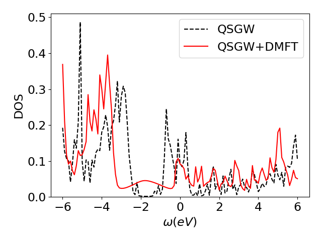Dos sr2ruo4

Spin susceptibility

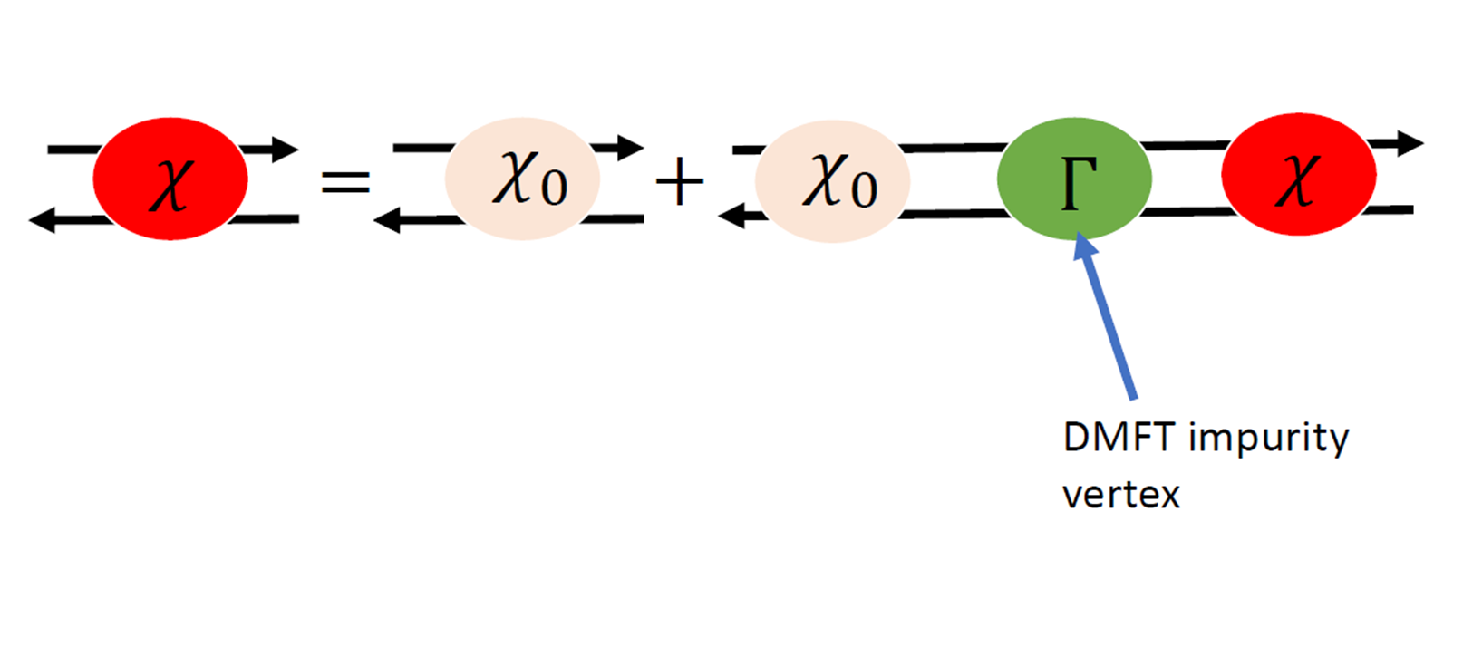BSE The spin susceptibility is obtained from the local vertex :

\chi(q,\Omega) = ( (\chi^0(q,\Omega))^{-1} - \Gamma(\Omega)) ^{-1}

The DMFT vertex is obtained from the local susceptibility :

\Gamma(\Omega) = (\chi^{0}(\Omega))^{-1} - \chi^{loc}(\Omega)^{-1}

impurity susceptibility

The local susceptibility is obtained from the two particle green function : $G^{(2)}_{\alpha\beta\gamma\delta}(\tau_1,\tau_2,\tau_3,\tau_4) = \langle\mathcal{T}_\tau c^\dagger_\alpha(\tau_1) c_\beta(\tau_2) c^\dagger_\gamma(\tau_3) c_\delta(\tau_4)\rangle.$

G^{(2)ph}_{\alpha\beta\gamma\delta}(\Omega;\nu,\nu') = \frac{1}{\beta}\int_0^\beta d\tau_1d\tau_2d\tau_3d\tau_4 \, e^{-i\nu\tau_1 + i(\nu+\Omega)\tau_2 - i(\nu'+\Omega)\tau_3 + i\nu'\tau_4} G^{(2)}_{\alpha\beta\gamma\delta}(\tau_1,\tau_2,\tau_3,\tau_4) \, .

\chi^{loc}_{\alpha\beta\gamma\delta}(\Omega,\nu,\nu) = G^{(2)ph}_{\alpha\beta\gamma\delta}(\Omega;\nu,\nu') - \chi^{0}_{\alpha\beta\gamma\delta}(\Omega;\nu,\nu')

The two-particles Green function has 1 bosonic frequency, 2 fermionic frequencies and 2 orbital indicies (formally 4 but we do not take into account off-diagonal terms in this tutorial). This quantity is computed by the TRIQS cthyb solver.

The first step is to modify the line with DMFT token on the ctrl file by :

DMFT NLOHI=16,42 BETA=30 NOMEGA=999 NOMF=50 NOMB=1

NOMF=50 : Number of fermionic frequencies to included in the local susceptibility
NOMB=1 : Number of bosinic frequencies to included in the local susceptibility

The computation of the two particle Green function severaly slows the solver. In this case, it is good to increase length_cycle in the para_triqs file and reduce n_cycles.

For the purpose of this tutorial, the local susceptibility has already be computed on a 240 cores machine with the following para_triqs.txt file :

U 4.5
J 1.0
n_warmup_cycles 100000
n_cycles 24000000
length_cycle 500
n_l 50

and run

mpirun -np 12 lmfdmft sr2ruo4  --ldadc~fn=dc --job=1 # makes sure that solver_input.h5 is updated
mpirun -np 12 lmtriqs sr2ruo4 --vertex

it takes around 9 hours.

In your folder, do :

cp extra/chiloc_1.h5 chiloc_1.h5

$\chi^{0}$

The $\chi^{0}(q,\Omega)$ is computed by lmfdmft.

$\chi^{0}(q,\Omega)$ can be computed on the 1 Brillouin zone or in a given q mesh. This q mesh has be given as follow : the first term is the size of the k mesh (should be equal to nkabc in the ctrl file (this option works for nkabc(1)=nkabs(2)=nkabs(3)). then on each line, q is given by :

$q = ik_1 Q_1 + ik_2 Q_2 + ik_2 Q_1$ where Q_1, Q_2, Q_3 are the reciprocal lattice vector and $ik_i \in [0..nk_i -1]$ .

In the case of Sr2RuO4 set up we have, Q1=(0.0, 1.0, 0.303848),Q2=(1.0,0.0, 0.303848),Q3=(1.0, 1.0,0.0). (It can be obtained at the beginning of the output of lmchk ctrl.sr2ruo4)

For instance, the following q list describes a q line along for $0$ to $Q_3$ on 9x9x9 q-mesh.

put the q-list in a file called “qlist” and then run :

lmfdmft sr2ruo4 -vnkabc=9 --ldadc~fn=dc --job=1 --chiloc --qlist
mpirun -np 12 lmfdmft sr2ruo4  --ldadc~fn=dc --job=1 # makes sure that solver_input.h5 is updated

Remark: To make $\chi^0$ and the full BZ, just remove the –qlist flag.

Finally the Bethe Salpeter equation is done by running :

susceptibility

it stores the susceptibility in a h5 format and in a txt file called chi_spin.txt :

\chi(\Omega,q) = \frac{1}{\beta} \sum_{\nu,\nu',a} \chi^{loc}_{\alpha \alpha \alpha \alpha}(\Omega,\nu,\nu')

#iq iom real(chi)    imag(chi)
0  13.3551597356 4.90070946787e-13
0  14.8699746786 2.31342722756e-12
0  17.6681324135 8.23262199153e-12
0  12.0345500361 8.8882197898e-12
0  7.24252562004 3.83866087065e-12
0  7.24252562004 4.06060740588e-12
0  12.0345500361 8.91117180046e-12
0  17.6681324135 8.94648059339e-12
0  14.8699746786 2.30697313105e-12

You can then plot it with your favorite program.

References

[1] K. Haule, C.H. Yee, and K. Kim. Dynamical mean field theory within the full-potential methods: Electronic structure of ceirin5, cecoin5, and cerhin5. Phys. Rev. B, 81:195107, 2010.

[2] Paolo Pisanti. A novel QSGW+DMFT method for the study of strongly correlated materials. PhD thesis, King’s College London, 2016.

[3] Lewin Boehnke et al. “Orthogonal polynomial representation of imaginary-time Green’s functions”. Physical Review B 84.7 (2011).

Impurity solver

Prepare Input folder and files

Definition of the correlated subspace

Projection window

Definition of the impurity

Double Counting

Solver parameters

First iteration

DMFT loop

Analyse of the result

Analytic continuation

Spectral function

Density of States

Spin susceptibility

impurity susceptibility

χ0\chi^{0}χ​0​​

References

$\chi^{0}$